Note

This page was generated from an Jupyter notebook that can be accessed from github.

MESMER-X workflow for annual maximum temperatures#

In this tutorial we use a conditional distribution to model the dependence of a climate variable on a global predictor using the approach from MESMER-X (Quilquaille et al., 2022). In this example we model annual maximum temperature with a normal distribution with a linear dependence on global mean temperature.

Note

We fit annual maximum data (i.e. a block maxima) using a normal distribution. This is not the appropriate distribution for this type of data but is used for illustrative purposes and speed.
A normal distribution with a linear dependence of the mean on a variable is equivalent to a linear regression with is much faster to use directly. Again, this is only for illustrative purposes.

import pathlib

import filefisher
import matplotlib.pyplot as plt
import xarray as xr

import mesmer
from mesmer.distrib import (
    ConditionalDistribution,
    Expression,
    ProbabilityIntegralTransform,
)

Calibration#

Configuration#

scenario = "ssp585"
target_name = "tasmax"
option_2ndfit = False
save_files = False

THRESHOLD_LAND = 1 / 3
REFERENCE_PERIOD = slice("1850", "1900")

esm = "IPSL-CM6A-LR"

cmip6_data_path = mesmer.example_data.cmip6_ng_path()

Load and prepare predictor and forcing data#

MESMER-X expectes the predictor and forcing data in the same format as MESMER and MESMER-M. First define helper functions to load data from the cmip6-ng example data archive.

Caution

In the original cmip6-ng archive annual tasmax archive is not the annual maximum temperature (TXx) but the annual mean daily maximum temperature. In MESMER’s example data archive the annual maximum is provided.

def find_files(variable, model, scenarios, member=None):

    CMIP_FILEFINDER = filefisher.FileFinder(
        path_pattern=str(cmip6_data_path / "{variable}/{time_res}/{resolution}"),
        file_pattern="{variable}_{time_res}_{model}_{scenario}_{member}_{resolution}.nc",
    )

    fc_scens_pred = CMIP_FILEFINDER.find_files(
        variable=variable,
        scenario=scenarios,
        model=model,
        member=member,
        resolution="g025",
        time_res="ann",
    )

    # only get the historical members that are also in the future scenarios, but only once
    unique_scen_members = fc_scens_pred.df.member.unique()

    fc_hist_pred = CMIP_FILEFINDER.find_files(
        variable=variable,
        scenario="historical",
        model=model,
        resolution="g025",
        time_res="ann",
        member=unique_scen_members,
    )

    fc_pred = fc_hist_pred.concat(fc_scens_pred)

    return fc_pred

def load_data(fc):
    data = xr.DataTree()

    scenarios = fc.df.scenario.unique().tolist()

    for scen in scenarios:
        # load data for each scenario
        data_scen = []

        for var in fc.df.variable.unique():
            files = fc.search(variable=var, scenario=scen)

            # load all members for a scenario
            members = []
            for fN, meta in files.items():
                time_coder = xr.coders.CFDatetimeCoder(use_cftime=True)
                ds = xr.open_dataset(fN, decode_times=time_coder)
                # drop unnecessary variables
                ds = ds.drop_vars(
                    ["height", "time_bnds", "file_qf", "area"], errors="ignore"
                )
                # assign member-ID as coordinate
                ds = ds.assign_coords({"member": meta["member"]})
                members.append(ds)

            # create a Dataset that holds each member along the member dimension
            data_var = xr.concat(members, dim="member")
            data_scen.append(data_var)

        data_scen = xr.merge(data_scen)
        data[scen] = xr.DataTree(data_scen)
    return data

load predictor data

fc_pred = find_files(variable="tas", model=esm, scenarios=scenario, member="r1i1p1f1")
tas = load_data(fc_pred)

# calculate anomalies w.r.t. the reference period
tas_anom = mesmer.anomaly.calc_anomaly(tas, reference_period=REFERENCE_PERIOD)

# calculate global mean
tas_glob_mean = mesmer.weighted.global_mean(tas_anom)

load target data

fc_targ = find_files(
    variable=target_name, model=esm, scenarios=scenario, member="r1i1p1f1"
)
targ_data_orig = load_data(fc_targ)

# calculate anomalies w.r.t. the reference period
targ_data = mesmer.anomaly.calc_anomaly(
    targ_data_orig, reference_period=REFERENCE_PERIOD
)

# mask ocean, Antarctica and stack the gridpoints
def mask_and_stack(ds, threshold_land):
    ds = mesmer.mask.mask_ocean_fraction(ds, threshold_land)
    ds = mesmer.mask.mask_antarctica(ds)
    ds = mesmer.grid.stack_lat_lon(ds, stack_dim="gridpoint")
    return ds


targ_data = mask_and_stack(targ_data, threshold_land=THRESHOLD_LAND)
pred_data = tas_glob_mean.copy()

also create weights, here samples are weighed by the inverse of their density to give rare samples more weight

weights = mesmer.weighted.get_weights_density(pred_data=pred_data)

pool data along the sample dimension

pooled_pred, pooled_targ, pooled_weights = mesmer.datatree.broadcast_and_pool_scen_ens(
    predictors=pred_data,
    target=targ_data,
    weights=weights,
)

Define the Expression and ConditionalDistribution#

The Expression defines the used distribution and the covariate structure and needs to be created as a string and has the following elements:

distribution: name of the desired distribution as written in scipy.stats
parameters: the parameters of the distribution as written in scipy (e.g. loc, scale, …)
predictors: predictors that the distribution will be conditional on, must be written as variable in python and surrounded by __ (e.g. __tas__)
coefficients: of the predictors and parameters, must be named c1, c2, …, c9.
mathematical operations: mathematical operations for the covariates are written as python code. Only functions from numpy (np.*) are supported.

Thus for the normal distribution with a linear dependence on global mean temperature (tas) this looks as follows:

expr = "norm(loc=c1 + c2 * __tas__, scale=c3)"

expr_name = "expr1"
expression_fit = Expression(expr, expr_name, boundaries_params={}, boundaries_coeffs={})

We then pass the Expression to the ConditionalDistribution class, which finds the best estimate of the coefficients for given climate model data.

distrib = ConditionalDistribution(expression=expression_fit)

Transform to standard normal distribution#

After fitting the coefficients the original data is transformed to a standard normal distribution, also removing the fitted linear trend:

# probability integral transform on non-stacked data for AR(1) process
target_expression = Expression("norm(loc=0, scale=1)", "normal_dist")

pit = ProbabilityIntegralTransform(
    distrib_orig=distrib,
    distrib_targ=ConditionalDistribution(target_expression),
)
transf_target = pit.transform(
    data=targ_data, target_name=target_name, preds_orig=pred_data, preds_targ=None
)

Local variability#

The resulting residuals constitute the local variability and are now treated the same way as in MESMER by fitting a local AR(1) process with a spatially correlated noise term.

# training of auto-regression with spatially correlated innovations
local_ar_params = mesmer.stats.fit_auto_regression_scen_ens(
    transf_target,
    ens_dim="member",
    dim="time",
    lags=1,
)

# estimate covariance matrix
# prep distance matrix
geodist = mesmer.geospatial.geodist_exact(
    lon=targ_data["historical"].lon, lat=targ_data["historical"].lat
)
# prep localizer
localisation_radii = range(3_500, 15_001, 250)
phi_gc_localizer = mesmer.stats.gaspari_cohn_correlation_matrices(
    geodist=geodist, localisation_radii=localisation_radii
)

pooled_transf_target = mesmer.datatree.pool_scen_ens(transf_target)


localized_ecov = mesmer.stats.find_localized_empirical_covariance(
    data=pooled_transf_target[target_name],
    weights=pooled_weights.weights.squeeze(),
    localizer=phi_gc_localizer,
    dim="sample",
    k_folds=30,
)

localized_ecov["localized_covariance_adjusted"] = mesmer.stats.adjust_covariance_ar1(
    localized_ecov.localized_covariance, local_ar_params.coeffs
)

Potentially save the params:

test_path = pathlib.Path("./output/")

file_end = f"{target_name}_{expr_name}_{esm}_{scenario}"
distrib_file = test_path / "distrib" / f"params_transform_distrib_{file_end}.nc"
local_ar_file = test_path / "local_variability" / f"params_local_AR_{file_end}.nc"
localized_ecov_file = (
    test_path / "local_variability" / f"params_localized_ecov_{file_end}.nc"
)

if save_files:
    # save the parameters
    transform_coeffs.to_netcdf(distrib_file)
    local_ar_params.to_netcdf(local_ar_file)
    localized_ecov.to_netcdf(localized_ecov_file)

Make emulations#

To generate emulations the workflow of the calibration is reversed, using the estimated parameters from above. Here, we use the same local annual mean temperatures to force the emulations, but temperatures from other models, scenarios, ensemble members or emulated annual local temperatures can be used as well.

Configuration#

# set some configuration parameters
n_realizations = 3
seed = 121638161038369005437100875176885634488
buffer = 10
esm = "IPSL-CM6A-LR"

targ_var = "tasmax"

Where the seed is random but constant (for reporducibility) and was created using

import secrets

secrets.randbits(64)

Load predictor data#

In contrast to above we concatenate the historical simulations and the projection.

cmip6_data_path = mesmer.example_data.cmip6_ng_path()

# load predictor data
path_tas = cmip6_data_path / "tas" / "ann" / "g025"

fN_hist = path_tas / f"tas_ann_{esm}_historical_r1i1p1f1_g025.nc"
fN_ssp585 = path_tas / f"tas_ann_{esm}_ssp585_r1i1p1f1_g025.nc"

time_coder = xr.coders.CFDatetimeCoder(use_cftime=True)
tas_hist = xr.open_dataset(fN_hist, decode_times=time_coder).drop_vars(
    ["height", "file_qf", "time_bnds"]
)
tas_ssp585 = xr.open_dataset(fN_ssp585, decode_times=time_coder).drop_vars(
    ["height", "file_qf", "time_bnds"]
)

# make global mean
# global_mean_dt = map_over_datasets(mesmer.weighted.global_mean)
tas_glob_mean_hist = mesmer.weighted.global_mean(tas_hist)
tas_glob_mean_ssp585 = mesmer.weighted.global_mean(tas_ssp585)

# concat
predictor = xr.concat([tas_glob_mean_hist, tas_glob_mean_ssp585], dim="time")

predictor = predictor - predictor.sel(time=REFERENCE_PERIOD).mean("time")


time = predictor.time

Load parameters#

This is skipped here because they are still defined from the calibration above.

# load data
# test_path = test_data_root_dir / "output" / targ_var / "one_scen_one_ens"

# load the parameters
# PARAM_FILEFINDER = FileFinder(
#     path_pattern=test_path / "test-params/{module}/",
#     file_pattern="params_{module}_{targ_var}_{expr_name}_{esm}_{scen}.nc",
# )

# distrib_file = PARAM_FILEFINDER.find_single_file(
#     module="distrib",
#     targ_var=targ_var,
#     expr_name=expr_name,
#     esm=esm,
#     scen=scenario,
# ).paths.pop()
# local_ar_file = PARAM_FILEFINDER.find_single_file(
#     module="local_trends",
#     targ_var=targ_var,
#     expr_name=expr_name,
#     esm=esm,
#     scen=scenario,
# ).paths.pop()
# localized_ecov_file = PARAM_FILEFINDER.find_single_file(
#     module="local_variability",
#     targ_var=targ_var,
#     expr_name=expr_name,
#     esm=esm,
#     scen=scenario,
# ).paths.pop()


# transform_coeffs = xr.open_dataset(distrib_file)

# local_ar_params = xr.open_dataset(local_ar_file)

# localized_ecov = xr.open_dataset(localized_ecov_file)

Create temporally and spatially corelated samples#

# generate realizations based on the auto-regression with spatially correlated innovations
transf_emus = mesmer.stats.draw_auto_regression_correlated(
    local_ar_params,
    localized_ecov.localized_covariance_adjusted,
    time=time,
    realisation=n_realizations,
    seed=seed,
    buffer=buffer,
)
transf_emus = transf_emus.rename({"samples": targ_var})

Transform samples back to the conditional distribution#

Initialize the conditional distribution with the calibrated values and the expression:

distrib_orig = ConditionalDistribution.from_dataset(transform_coeffs)

define a standard normal distribution and the probability integral transform:

# back-transform the realizations
expr_tranf = Expression("norm(loc=0, scale=1)", "standard_normal")
distrib_transf = ConditionalDistribution(expr_tranf)

back_pit = ProbabilityIntegralTransform(
    distrib_orig=distrib_transf,
    distrib_targ=distrib_orig,
)

and fially back-transform the realizations

emus = back_pit.transform(
    data=transf_emus, target_name=targ_var, preds_orig=None, preds_targ=predictor
)

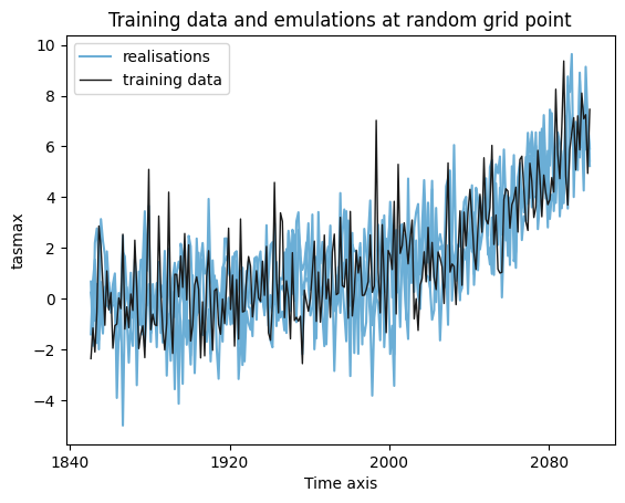
Illustration#

gridpoint = 0

f, ax = plt.subplots()

emus.tasmax.isel(gridpoint=gridpoint).plot.line(
    ax=ax, x="time", color="#6baed6", add_legend=False
)

ax.plot([], [], label="realisations", color="#6baed6")

pooled_targ.tasmax.isel(gridpoint=gridpoint).plot(
    ax=ax, x="time", color="0.1", label="training data", lw=1
)

ax.legend()

ax.set_title("Training data and emulations at random grid point")

Text(0.5, 1.0, 'Training data and emulations at random grid point')

../_images/c1b35becf26d20c502c00242c3741a6fedb5627977d97a19fc2793c4e1685e24.png

MESMER-X workflow for annual maximum temperatures

Contents

MESMER-X workflow for annual maximum temperatures#

Calibration#

Configuration#

Load and prepare predictor and forcing data#

Define the Expression and ConditionalDistribution#

Fit conditional distribution#

Transform to standard normal distribution#

Local variability#

Make emulations#

Configuration#

Load predictor data#

Load parameters#

Create temporally and spatially corelated samples#

Transform samples back to the conditional distribution#

Illustration#