Note
This page was generated from an Jupyter notebook that can be accessed from github.
MESMER-M workflow for multiple scenarios#
Training and emulation of monthly local temperature from yearly local temperature for multiple scenarios and ensemble members. We use an example data set on a coarse grid. This roughly follows the approach outlined in Nath et al. (2022).
MESMER-M trains the local monthly temperature using the local annual temperature (i.e. the temperature from the same grid point) as forcing. This is different from MESMER which uses global mean values as predictors for where local annual mean temperatures. Training MESMER-M consists of 4 steps:
harmonic model: fit the seasonal cycle with a harmonic model
power transformer: make the resulting residuals more normal by using a Yeo-Johnson transformation
cyclo-stationary AR(1) process: the monthly residuals are assumed to follow a cyclo-stationary AR(1) process, where one months value depends on the previous one
local variability: estimate parameters needed to generate local variability
This example can be extended to more scenarios, ensemble members and higher resolution data. See also the MESMER-M calibration and emulation tests in tests/integration/.
import filefisher
import matplotlib.pyplot as plt
import pandas as pd
import scipy as sp
import xarray as xr

import mesmer
Calibration#
Configuration#
LOCALISATION_RADII = list(range(7_500, 12_501, 500))
THRESHOLD_LAND = 1 / 3
REFERENCE_PERIOD = slice("1850", "1900")
# define model and scenarios
model = "IPSL-CM6A-LR"
scenarios = ["ssp126", "ssp585"]

# path of the example data
cmip6_data_path = mesmer.example_data.cmip6_ng_path(relative=True)
Load Data for training the emulator#
We load monthly and annual mean temperatures.
CMIP_FILEFINDER = filefisher.FileFinder(
    path_pattern=cmip6_data_path / "{variable}/{time_res}/{resolution}",
    file_pattern="{variable}_{time_res}_{model}_{scenario}_{member}_{resolution}.nc",
)
Find annual data:
fc_scens_y = CMIP_FILEFINDER.find_files(
    variable="tas", scenario=scenarios, model=model, resolution="g025", time_res="ann"
)

# get the historical members that are also in the future scenarios, but only once
unique_scen_members_y = fc_scens_y.df.member.unique()

fc_hist_y = CMIP_FILEFINDER.find_files(
    variable="tas",
    scenario="historical",
    model=model,
    resolution="g025",
    time_res="ann",
    member=unique_scen_members_y,
)

fc_all_y = fc_hist_y.concat(fc_scens_y)
fc_all_y.df
| variable | time_res | resolution | model | scenario | member | |
|---|---|---|---|---|---|---|
| path | ||||||
| ../data/cmip6-ng/tas/ann/g025/tas_ann_IPSL-CM6A-LR_historical_r1i1p1f1_g025.nc | tas | ann | g025 | IPSL-CM6A-LR | historical | r1i1p1f1 |
| ../data/cmip6-ng/tas/ann/g025/tas_ann_IPSL-CM6A-LR_historical_r2i1p1f1_g025.nc | tas | ann | g025 | IPSL-CM6A-LR | historical | r2i1p1f1 |
| ../data/cmip6-ng/tas/ann/g025/tas_ann_IPSL-CM6A-LR_ssp126_r1i1p1f1_g025.nc | tas | ann | g025 | IPSL-CM6A-LR | ssp126 | r1i1p1f1 |
| ../data/cmip6-ng/tas/ann/g025/tas_ann_IPSL-CM6A-LR_ssp585_r1i1p1f1_g025.nc | tas | ann | g025 | IPSL-CM6A-LR | ssp585 | r1i1p1f1 |
| ../data/cmip6-ng/tas/ann/g025/tas_ann_IPSL-CM6A-LR_ssp585_r2i1p1f1_g025.nc | tas | ann | g025 | IPSL-CM6A-LR | ssp585 | r2i1p1f1 |
Find monthly data:
fc_scens_m = CMIP_FILEFINDER.find_files(
    variable="tas", scenario=scenarios, model=model, resolution="g025", time_res="mon"
)

# get the historical members that are also in the future scenarios, but only once
unique_scen_members_m = fc_scens_y.df.member.unique()

fc_hist_m = CMIP_FILEFINDER.find_files(
    variable="tas",
    scenario="historical",
    model=model,
    resolution="g025",
    time_res="mon",
    member=unique_scen_members_m,
)

fc_all_m = fc_hist_m.concat(fc_scens_m)
fc_all_m.df
| variable | time_res | resolution | model | scenario | member | |
|---|---|---|---|---|---|---|
| path | ||||||
| ../data/cmip6-ng/tas/mon/g025/tas_mon_IPSL-CM6A-LR_historical_r1i1p1f1_g025.nc | tas | mon | g025 | IPSL-CM6A-LR | historical | r1i1p1f1 |
| ../data/cmip6-ng/tas/mon/g025/tas_mon_IPSL-CM6A-LR_historical_r2i1p1f1_g025.nc | tas | mon | g025 | IPSL-CM6A-LR | historical | r2i1p1f1 |
| ../data/cmip6-ng/tas/mon/g025/tas_mon_IPSL-CM6A-LR_ssp126_r1i1p1f1_g025.nc | tas | mon | g025 | IPSL-CM6A-LR | ssp126 | r1i1p1f1 |
| ../data/cmip6-ng/tas/mon/g025/tas_mon_IPSL-CM6A-LR_ssp585_r1i1p1f1_g025.nc | tas | mon | g025 | IPSL-CM6A-LR | ssp585 | r1i1p1f1 |
| ../data/cmip6-ng/tas/mon/g025/tas_mon_IPSL-CM6A-LR_ssp585_r2i1p1f1_g025.nc | tas | mon | g025 | IPSL-CM6A-LR | ssp585 | r2i1p1f1 |
This found 1 ensemble member for SSP1-2.6 and two for SSP5-8.5 and the corresponding ones in the historical scenario.
To load the data we write a small helper function that loads the data into a DataTree (where each node is a scenario):
def load_data(filecontainer):

    out = xr.DataTree()

    scenarios = filecontainer.df.scenario.unique().tolist()

    # load data for each scenario
    for scen in scenarios:
        files = filecontainer.search(scenario=scen)

        # load all members for a scenario
        members = []
        for fN, meta in files.items():
            time_coder = xr.coders.CFDatetimeCoder(use_cftime=True)
            ds = xr.open_dataset(fN, decode_times=time_coder)
            # drop unnecessary variables
            ds = ds.drop_vars(["height", "time_bnds", "file_qf"], errors="ignore")
            # assign member-ID as coordinate
            ds = ds.assign_coords({"member": meta["member"]})
            members.append(ds)

        # create a Dataset that holds each member along the member dimension
        scen_data = xr.concat(members, dim="member")
        # put the scenario dataset into the DataTree
        out[scen] = xr.DataTree(scen_data)

    return out
Load annual and monthly data:
tas_y_orig = load_data(fc_all_y)
tas_m_orig = load_data(fc_all_m)
This results in two DataTree objects, with 3 nodes, one for each scenario (click on Groups to see the individual Datasets for the three scenarios):
tas_y_orig
<xarray.DatasetView> Size: 0B
Dimensions:  ()
Data variables:
*empty*Preprocessing#
Calculate anomalies w.r.t the reference period
tas_anoms_y = mesmer.anomaly.calc_anomaly(tas_y_orig, reference_period=REFERENCE_PERIOD)
tas_anoms_m = mesmer.anomaly.calc_anomaly(tas_m_orig, reference_period=REFERENCE_PERIOD)
We only use land grid points and exclude Antarctica. The 3D data with dimensions ('time', 'lat', 'lon') is stacked to 2D data with dimensions ('time', 'gridcell'):
def mask_and_stack(ds, threshold_land):
    ds = mesmer.mask.mask_ocean_fraction(ds, threshold_land)
    ds = mesmer.mask.mask_antarctica(ds)
    ds = mesmer.grid.stack_lat_lon(ds)
    return ds
tas_y = mask_and_stack(tas_anoms_y, threshold_land=THRESHOLD_LAND)
tas_m = mask_and_stack(tas_anoms_m, threshold_land=THRESHOLD_LAND)
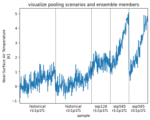
Finally we pool all scenarios, and ensemble members into one dataset:
tas_pooled_y = mesmer.datatree.pool_scen_ens(tas_y)
tas_pooled_m = mesmer.datatree.pool_scen_ens(tas_m)
Here we get a Dataset where scenario, member, and time is pooled along a sample dimension. scenario, member, and time are kept as non-dimension coordinates, so we still know where each point comes from.
tas_pooled_y
<xarray.Dataset> Size: 585kB
Dimensions:   (gridcell: 118, sample: 588)
Coordinates:
    scenario  (sample) object 5kB 'historical' 'historical' ... 'ssp585'
    time      (sample) object 5kB 1850-07-01 06:00:00 ... 2100-07-01 06:00:00
    member    (sample) <U8 19kB 'r1i1p1f1' 'r1i1p1f1' ... 'r2i1p1f1' 'r2i1p1f1'
    lat       (gridcell) float64 944B -49.5 -40.5 -31.5 -31.5 ... 76.5 76.5 76.5
    lon       (gridcell) float64 944B 288.0 288.0 18.0 ... 306.0 324.0 342.0
Dimensions without coordinates: gridcell, sample
Data variables:
    tas       (sample, gridcell) float64 555kB -0.1548 -0.1209 ... 13.42 16.16
Attributes: (12/56)
    CDI:                       Climate Data Interface version 1.9.9 (https://...
    source:                    IPSL-CM6A-LR (2017):  atmos: LMDZ (NPv6, N96; ...
    institution:               Institut Pierre Simon Laplace, Paris 75252, Fr...
    Conventions:               CF-1.7 CMIP-6.2
    history:                   Thu Mar 18 19:05:09 2021: cdo remapbil,r20x20 ...
    creation_date:             2018-07-11T07:36:34Z
    ...                        ...
    realization_index:         1
    NCO:                       "4.6.0"
    cmip6-ng:                  \ncontact = cmip6-archive@env.ethz.ch\ndescrip...
    original_file_names:       /net/atmos/data/cmip6/historical/Amon/tas/IPSL...
    original_file_hash_codes:  7264c228560257b32d44dcc611d92976da7214af7e8795...
CDO: Climate Data Operators version 1.9.9 (https://...def visualize_pooling(data):
mi = pd.MultiIndex.from_arrays([data["scenario"].values, data["member"].values])
f, ax = plt.subplots()
data.plot()
xticks, xticklabels = [], []
for i in mi.unique():
loc = mi.get_loc(i)
center = loc.start + (loc.stop - loc.start) / 2
plt.axvline(loc.stop, color="0.1", lw=0.5)
xticklabels.append("\n".join(i))
xticks.append(center)
ax.set_xticks(xticks)
ax.set_xticklabels(xticklabels)
ax.xaxis.set_tick_params(length=0)
ax.set_title("visualize pooling scenarios and ensemble members")
ax.set_xlim(0, data.sample.size)
visualize_pooling(tas_pooled_y.tas.isel(gridcell=0))
Fit the harmonic model#
With all the data preparation done we can now calibrate the different steps of MESMER-M. First we fit the seasonal cycle with a harmonic model which can vary with local annual mean temperature (fourier regression). This step removes the annual mean and determines the optimal order and the coefficients of the harmonic model.
harmonic_model_fit = mesmer.stats.fit_harmonic_model(tas_pooled_y.tas, tas_pooled_m.tas)
harmonic_model_fit
<xarray.Dataset> Size: 7MB
Dimensions:         (gridcell: 118, coeff: 24, sample: 7056)
Coordinates:
    lat             (gridcell) float64 944B -49.5 -40.5 -31.5 ... 76.5 76.5 76.5
    lon             (gridcell) float64 944B 288.0 288.0 18.0 ... 324.0 342.0
  * coeff           (coeff) int64 192B 0 1 2 3 4 5 6 7 ... 17 18 19 20 21 22 23
    scenario        (sample) object 56kB 'historical' 'historical' ... 'ssp585'
    time            (sample) object 56kB 1850-01-16 12:00:00 ... 2100-12-16 1...
    member          (sample) <U8 226kB 'r1i1p1f1' 'r1i1p1f1' ... 'r2i1p1f1'
Dimensions without coordinates: gridcell, sample
Data variables:
    selected_order  (gridcell) int64 944B 3 3 3 2 2 3 3 4 3 ... 2 4 4 3 3 3 2 4
    coeffs          (gridcell, coeff) float64 23kB -0.04407 4.653 ... nan nan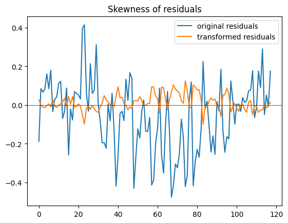
residuals (sample, gridcell) float64 7MB -0.6276 -1.249 ... -1.833Train the power transformer#
The residuals are not necessarily symmetric - make them more normal using a Yeo-Johnson transformation. For performance reasons we use a constant \(\lambda\) here. Originally, the parameter \(\lambda\) is modelled with a logistic regression using local annual mean temperature as covariate (Nath et al., 2022). Currently "constant" and "logistic" covariance structures are implemented - further options could be implemented and tested.
# yj_transformer = mesmer.stats.YeoJohnsonTransformer("logistic")

yj_transformer = mesmer.stats.YeoJohnsonTransformer("constant")

pt_coefficients = yj_transformer.fit(tas_pooled_y.tas, harmonic_model_fit.residuals)
transformed_resids = yj_transformer.transform(
    tas_pooled_y.tas,
    harmonic_model_fit.residuals,
    pt_coefficients,
)
To illustrate this we plot the skewness of the original and the transformed residuals:
f, ax = plt.subplots()

ax.plot(
    sp.stats.skew(harmonic_model_fit.residuals, axis=0),
    label="original residuals",
)
ax.plot(
    sp.stats.skew(transformed_resids.transformed.T, axis=0),
    label="transformed residuals",
)

ax.axhline(0, lw=0.5, color="0.1")
ax.legend()
ax.set_title("Skewness of residuals")
Text(0.5, 1.0, 'Skewness of residuals')
Fit cyclo-stationary AR(1) process#
The monthly residuals are now assumed to follow a cyclo-stationary AR(1) process, where e.g. the July residuals depend on the ones from June and the ones of June on May’s with distinct parameters. Because the first timestep has no previous one, we loose one time step of the residuals.
ar1_fit = mesmer.stats.fit_auto_regression_monthly(transformed_resids.transformed)
ar1_fit
<xarray.Dataset> Size: 7MB
Dimensions:    (month: 12, gridcell: 118, sample: 7055)
Coordinates:
    lat        (gridcell) float64 944B -49.5 -40.5 -31.5 ... 76.5 76.5 76.5
    lon        (gridcell) float64 944B 288.0 288.0 18.0 ... 306.0 324.0 342.0
  * month      (month) int64 96B 1 2 3 4 5 6 7 8 9 10 11 12
    scenario   (sample) object 56kB 'historical' 'historical' ... 'ssp585'
    time       (sample) object 56kB 1850-02-15 00:00:00 ... 2100-12-16 12:00:00
    member     (sample) <U8 226kB 'r1i1p1f1' 'r1i1p1f1' ... 'r2i1p1f1'
Dimensions without coordinates: gridcell, sample
Data variables:
    slope      (month, gridcell) float64 11kB 0.1944 0.1468 ... -0.06053 0.08392
    intercept  (month, gridcell) float64 11kB -0.05807 -0.1008 ... 0.01934
residuals (gridcell, sample) float64 7MB -0.04294 0.1836 ... -2.449 -1.651Find localized empirical covariance#
Finally, we determine the localized empirical spatial covariance for each month separately:
geodist = mesmer.geospatial.geodist_exact(tas_y.historical.lon, tas_y.historical.lat)

phi_gc_localizer = mesmer.stats.gaspari_cohn_correlation_matrices(
    geodist, localisation_radii=LOCALISATION_RADII
)
weights = mesmer.weighted.equal_scenario_weights_from_datatree(tas_anoms_m)
weights = mesmer.datatree.pool_scen_ens(weights)

# because ar1_fit.residuals lost the first ts, we have to remove it here as well
weights = weights.isel(sample=slice(1, None))
weights
<xarray.Dataset> Size: 395kB
Dimensions:   (sample: 7055)
Coordinates:
    scenario  (sample) object 56kB 'historical' 'historical' ... 'ssp585'
    time      (sample) object 56kB 1850-02-15 00:00:00 ... 2100-12-16 12:00:00
    member    (sample) <U8 226kB 'r1i1p1f1' 'r1i1p1f1' ... 'r2i1p1f1' 'r2i1p1f1'
Dimensions without coordinates: sample
Data variables:
weights (sample) float64 56kB 0.5 0.5 0.5 0.5 0.5 ... 0.5 0.5 0.5 0.5 0.5The more samples we pass to find_localized_empirical_covariance_monthly, the estimated localisation radius becomes larger. You may want to pass more LOCALISATION_RADII than we do here (however, the function warns if either the smallest or largest localisation radius is chosen).
localized_ecov = mesmer.stats.find_localized_empirical_covariance_monthly(
    ar1_fit.residuals,
    weights.weights,
    phi_gc_localizer,
    dim="time",
    k_folds=30,
)
localized_ecov
<xarray.Dataset> Size: 3MB
Dimensions:               (month: 12, gridcell_i: 118, gridcell_j: 118)
Coordinates:
  * month                 (month) int64 96B 1 2 3 4 5 6 7 8 9 10 11 12
Dimensions without coordinates: gridcell_i, gridcell_j
Data variables:
    localization_radius   (month) int64 96B 11000 10500 10000 ... 10000 10500
    covariance            (month, gridcell_i, gridcell_j) float64 1MB 0.723 ....
localized_covariance (month, gridcell_i, gridcell_j) float64 1MB 0.723 ....Saving#
time coordinate#
We need to get the original time coordinate to be able to validate our results later on. If it is not needed to align the final emulations with the original data, this can be omitted, the time coordinates can later be generated for example with
monthly_time = xr.cftime_range("1850-01-01", "2100-12-31", freq="MS", calendar="gregorian")
monthly_time = xr.DataArray(monthly_time, dims="time", coords={"time": monthly_time})
# extract and save time coordinate
hist_time = tas_m.historical.time
scen_time = tas_m.ssp585.time
m_time = xr.concat([hist_time, scen_time], dim="time")

# TODO
# save the parameters to a file
# harmonic_model_fit
# pt_coefficients
# ar1_fit
# localized_ecov
# m_time
Make emulations#
To generate emulations the workflow of the calibration is reversed, using the estimated parameters from above. Here, we use the same local annual mean temperatures to force the emulations, but temperatures from other models, scenarios, ensemble members or emulated annual local temperatures can be used as well.
# # Re-import necessary libraries
# import matplotlib.pyplot as plt
# import xarray as xr

# import mesmer
Configuration#
# parameters
NR_EMUS = 10
BUFFER = 20
# REF_PERIOD = slice("1850", "1900")
Random number seed#
The seed determines the initial state for the random number generator. To avoid generating the same noise for different models and scenarios different seeds are required for each individual paring. For reproducibility the seed needs to be the same for any subsequent draw of the same emulator. To avoid human chosen standard seeds (e.g. 0, 1234) its recommended to also randomly generate the seeds and save them for later, using
import secrets
secrets.randbits(128)
# random but constant
SEED = 172968389139962348981869773740375508145
Load data needed for emulations#
# TODO: load the parameters from a file
# in this example notebook we directly use the calibration from above
# TODO: load yearly temperature
# in this example we are using the original yearly temperature for demonstration
Preprocessing#
# preprocess tas
# ref = tas_y.sel(time=REF_PERIOD).mean("time", keep_attrs=True)
# tas_y = tas_y - ref
# tas_stacked_y = mask_and_stack(tas_y, threshold_land=THRESHOLD_LAND)
# get the original grid for transforming back later
grid_orig = tas_anoms_y["historical"].to_dataset()[["lat", "lon"]]
Concatenate historical and scenario annual mean temperature timeseries. We use this as predictor for our emulations.
yearly_predictor = xr.concat(
    [
        tas_y.historical.tas.sel(member="r1i1p1f1"),
        tas_y.ssp585.tas.sel(member="r1i1p1f1"),
    ],
    dim="time",
)
Generate emulations#
To generate emulations we have to invert the steps done in the calibration.
# generate monthly data with harmonic model
monthly_harmonic_emu = mesmer.stats.predict_harmonic_model(
    yearly_predictor, harmonic_model_fit.coeffs, m_time
)

# generate variability around 0 with AR(1) model
local_variability_transformed = mesmer.stats.draw_auto_regression_monthly(
    ar1_fit,
    localized_ecov.localized_covariance,
    time=m_time,
    n_realisations=NR_EMUS,
    seed=SEED,
    buffer=BUFFER,
)

# invert the power transformation
yj_transformer = mesmer.stats.YeoJohnsonTransformer("constant")
local_variability_inverted = yj_transformer.inverse_transform(
    yearly_predictor,
    local_variability_transformed.samples,
    pt_coefficients,
)

# add the local variability to the monthly harmonic
emulations = monthly_harmonic_emu + local_variability_inverted.inverted
emulations
<xarray.DataArray (time: 3012, gridcell: 118, realisation: 10)> Size: 28MB
array([[[  4.71933552,   3.19453385,   5.55971229, ...,   3.53583741,
           3.07968852,   4.83855914],
        [  6.08102713,   4.47278448,   5.80856711, ...,   3.97114309,
           4.25836007,   6.66574778],
        [  3.22420126,   4.42569327,   5.02006883, ...,   4.70094755,
           4.19620652,   3.15460483],
        ...,
        [-14.36493511, -14.08182641, -11.09121839, ..., -12.08415207,
         -14.15155807, -16.93798278],
        [-16.13098318, -17.73577325,  -9.6149607 , ..., -12.69205604,
         -19.25888759, -14.44866455],
        [-16.16861358, -15.88550476, -11.25557184, ..., -11.11201536,
         -15.56585009,  -7.29204366]],

       [[  4.48380178,   5.12766377,   4.56309968, ...,   3.8360322 ,
           5.25166695,   3.86276331],
        [  6.10225199,   6.37292685,   4.93442445, ...,   5.4030034 ,
           7.98633604,   5.77929225],
        [  4.81451917,   5.5286049 ,   5.16768035, ...,   5.3128797 ,
           5.61305701,   4.77722429],
...
        [  3.24460364,   3.26958029,   4.80969676, ...,   4.6153487 ,
           3.95723251,   6.54548137],
        [  2.69145111,   2.1366067 ,   3.7489604 , ...,   4.4963506 ,
           6.9024826 ,   6.97475093],
        [ 21.636935  ,  14.51010995,  16.71091134, ...,  19.1729279 ,
          17.71089084,  12.84282912]],

       [[  8.33495891,   6.6318643 ,   8.02679003, ...,   6.49548798,
           8.83021519,   7.84355059],
        [ 10.14076982,   8.34635754,  10.00186498, ...,   8.59491647,
          10.86391849,   9.28815237],
        [  8.18063192,   7.20274524,   7.94618335, ...,   7.56771585,
           7.1358091 ,   8.06112174],
        ...,
        [ -0.29584109,   1.06735266,  -5.73758839, ...,  -4.36359569,
          -0.80116777,  -2.01771841],
        [ -2.17666204,  -1.46807633,  -5.31560253, ...,  -5.80926704,
          -2.37928138,  -5.41091808],
        [ 13.38347722,  14.75829661,   9.86888608, ...,  13.05124836,
          12.44905657,  16.0469594 ]]], shape=(3012, 118, 10))
Coordinates:
    member   <U8 32B 'r1i1p1f1'
    lat      (gridcell) float64 944B -49.5 -40.5 -31.5 -31.5 ... 76.5 76.5 76.5
    lon      (gridcell) float64 944B 288.0 288.0 18.0 ... 306.0 324.0 342.0
  * time     (time) object 24kB 1850-01-16 12:00:00 ... 2100-12-16 12:00:00
Dimensions without coordinates: gridcell, realisationSaving and/or Analysis#
# TODO
# save
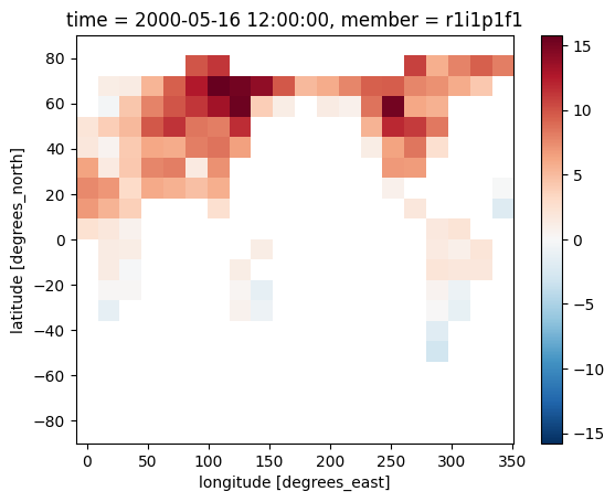
The emulations are still stacked - to get back to the lat/ lon grid we have to unstack them:
# unstack to original grid
emulations_unstacked = mesmer.grid.unstack_lat_lon_and_align(emulations, grid_orig)
We can then visualize a random month of the emulated temperature fields - e.g. May 2000:
emulations_unstacked.isel(realisation=0).sel(time="2000-05").plot()
<matplotlib.collections.QuadMesh at 0x7060f0344200>
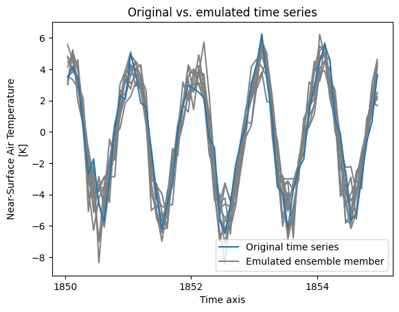
or compare the original monthly time series to our emulations.
gridcell = 0
time_period = slice(None, 60)


f, ax = plt.subplots()

# loop realisations
for i in range(10):
    d = emulations.isel(gridcell=gridcell, realisation=i, time=time_period)
    d.plot(ax=ax, color="0.5")


# show original time series
d = tas_m["historical"].sel(member="r1i1p1f1")
d = d.isel(gridcell=gridcell, time=time_period)
d.tas.plot(color="#1f78b4", label="Original time series")

# legend entry
ax.plot([], [], color="0.5", label="Emulated ensemble member")

ax.set_title("Original vs. emulated time series")

plt.legend()
<matplotlib.legend.Legend at 0x7060f0da86e0>