Note
This page was generated from an Jupyter notebook that can be accessed from github.
Calibrating MESMER on multiple scenarios#
This tutorial shows how to calibrate the parameters for MESMER on an example dataset of coarse regridded ESM output for multiple climate change scenarios. We calibrate the parameters for MESMER using three scenarios: a historical, a low emission (SSP1-2.6), and a high emission (SSP5-8.5) scenario, where SSP5-8.5 includes several ensemble members. You can find the basics of the MESMER approach in Beusch et al. (2020) and the multi-sceario approach in Beusch et al. (2022). Training MESMER consists of four steps:
global trend: compute the global temperature trend, including the volcanic influence on historical trends
global variablity: estimating the parameters to generate global variability
local trend: estimate parameters to translate global mean temperature (including global variability) into local temperature
local variability: estimate parameters needed to generate local variability
This example can be extended to more scenarios, ensemble members and higher resolution data. See also the mesmer calibration test in tests/integration/.
import pathlib

import cartopy.crs as ccrs
import filefisher
import matplotlib.pyplot as plt
import xarray as xr

import mesmer
Load data#
MESMER expects a specific data format. Data from each scenario should be a node (or group) on an xr.DataTree (more on this below) e.g.:
<xarray.DataTree>
Group: /
├── Group: /historical
|    ...
├── Group: /ssp126
|    ...
Each scenario is a xr.Dataset with 4 dimensions: member, time, lat, lon. Below we show one way to load data such that it conforms to the desired format. We load data from the cmip6-ng (“new generation”) repository. This data has undergone a small reformatting from the original cmip6 archive. For the sake of computational speed we also load data which has been regridded to a coarse resolution. Loading the data can be adapted to the data format you are most used to - as long as the final output has the desired format.
MESMER is Earth System Model specific, aiming to reproduce the behaviour of one ESM. Here we train on the CMIP6 output of the model IPSL-CM6A-LR.
model = "IPSL-CM6A-LR"
We use the library filefisher to search all files in the cmip6-ng archive for the model and scenarios we want to use. Filefisher can search through paths for given file patterns. It returns all paths matching the pattern such that you can load the files in the next step.
Here, we want to find all files that have data for annual near surface temperature ("tas") for the used model and the future scenarios ssp126 and ssp585. Next, we search for the historical data that match the members found for the two future scenarios.
# mesmer provides example data under "./data/cmip6-ng"
cmip_data_path = mesmer.example_data.cmip6_ng_path(relative=True)

CMIP_FILEFINDER = filefisher.FileFinder(
    path_pattern=cmip_data_path / "{variable}/{time_res}/{resolution}",
    file_pattern="{variable}_{time_res}_{model}_{scenario}_{member}_{resolution}.nc",
)
CMIP_FILEFINDER
<FileFinder>
path_pattern: '../data/cmip6-ng/{variable}/{time_res}/{resolution}/'
file_pattern: '{variable}_{time_res}_{model}_{scenario}_{member}_{resolution}.nc'

keys: 'member', 'model', 'resolution', 'scenario', 'time_res', 'variable'
Search data for ssp126 and ssp585 - we find one and two ensemble members, respectively:
scenarios = ["ssp126", "ssp585"]

keys = {"variable": "tas", "model": model, "resolution": "g025", "time_res": "ann"}

fc_scens = CMIP_FILEFINDER.find_files(scenario=scenarios, keys=keys)
fc_scens.df
| variable | time_res | resolution | model | scenario | member | |
|---|---|---|---|---|---|---|
| path | ||||||
| ../data/cmip6-ng/tas/ann/g025/tas_ann_IPSL-CM6A-LR_ssp126_r1i1p1f1_g025.nc | tas | ann | g025 | IPSL-CM6A-LR | ssp126 | r1i1p1f1 |
| ../data/cmip6-ng/tas/ann/g025/tas_ann_IPSL-CM6A-LR_ssp585_r1i1p1f1_g025.nc | tas | ann | g025 | IPSL-CM6A-LR | ssp585 | r1i1p1f1 |
| ../data/cmip6-ng/tas/ann/g025/tas_ann_IPSL-CM6A-LR_ssp585_r2i1p1f1_g025.nc | tas | ann | g025 | IPSL-CM6A-LR | ssp585 | r2i1p1f1 |
We also need to find the same ensemble members in the historical data, such that we end up with five files we need to load:
# get the historical members that are also in the future scenarios, but only once
members = fc_scens.df.member.unique()

fc_hist = CMIP_FILEFINDER.find_files(scenario="historical", member=members, keys=keys)

fc_all = fc_hist.concat(fc_scens)
fc_all.df
| variable | time_res | resolution | model | scenario | member | |
|---|---|---|---|---|---|---|
| path | ||||||
| ../data/cmip6-ng/tas/ann/g025/tas_ann_IPSL-CM6A-LR_historical_r1i1p1f1_g025.nc | tas | ann | g025 | IPSL-CM6A-LR | historical | r1i1p1f1 |
| ../data/cmip6-ng/tas/ann/g025/tas_ann_IPSL-CM6A-LR_historical_r2i1p1f1_g025.nc | tas | ann | g025 | IPSL-CM6A-LR | historical | r2i1p1f1 |
| ../data/cmip6-ng/tas/ann/g025/tas_ann_IPSL-CM6A-LR_ssp126_r1i1p1f1_g025.nc | tas | ann | g025 | IPSL-CM6A-LR | ssp126 | r1i1p1f1 |
| ../data/cmip6-ng/tas/ann/g025/tas_ann_IPSL-CM6A-LR_ssp585_r1i1p1f1_g025.nc | tas | ann | g025 | IPSL-CM6A-LR | ssp585 | r1i1p1f1 |
| ../data/cmip6-ng/tas/ann/g025/tas_ann_IPSL-CM6A-LR_ssp585_r2i1p1f1_g025.nc | tas | ann | g025 | IPSL-CM6A-LR | ssp585 | r2i1p1f1 |
Now we load all the files we found into a DataTree, a data structure provided by xarray. It is a container to hold xarray Dataset objects that are not alignable. This is useful for us since we have historical and future data, which have different time coordinates. Moreover, the scenarios may also have different numbers of members (as e.g., SSP1-2.6, which only has one). Thus, we store the data of each scenario in a Dataset with all its ensemble members along a member dimension. Then we store all the scenario datasets in one DataTree node. The DataTree allows us to perform computations on each of the scenarios separately.
We define a helper function to load the data from the cmip6_ng example data repository:
def load_data(filecontainer):

    out = xr.DataTree()

    scenarios = filecontainer.df.scenario.unique().tolist()

    # load data for each scenario
    for scen in scenarios:
        files = filecontainer.search(scenario=scen)

        # load all members for a scenario
        members = []
        for fN, meta in files.items():
            time_coder = xr.coders.CFDatetimeCoder(use_cftime=True)
            ds = xr.open_dataset(fN, decode_times=time_coder)
            # drop unnecessary variables
            ds = ds.drop_vars(["height", "time_bnds", "file_qf"], errors="ignore")
            # assign member-ID as coordinate
            ds = ds.assign_coords({"member": meta["member"]})
            members.append(ds)

        # create a Dataset that holds each member along the member dimension
        scen_data = xr.concat(members, dim="member")
        # put the scenario dataset into the DataTree
        out[scen] = xr.DataTree(scen_data)

    return out
dt = load_data(fc_all)
dt
<xarray.DatasetView> Size: 0B
Dimensions:  ()
Data variables:
*empty*<xarray.DatasetView> Size: 1MB Dimensions: (member: 2, time: 165, lat: 20, lon: 20) Coordinates: * time (time) object 1kB 1850-07-01 06:00:00 ... 2014-07-01 06:00:00 * lon (lon) float64 160B 0.0 18.0 36.0 54.0 ... 288.0 306.0 324.0 342.0 * lat (lat) float64 160B -85.5 -76.5 -67.5 -58.5 ... 58.5 67.5 76.5 85.5 * member (member) <U8 64B 'r1i1p1f1' 'r2i1p1f1' Data variables: tas (member, time, lat, lon) float64 1MB 226.3 225.0 ... 258.4 259.6 Attributes: (12/56) CDI: Climate Data Interface version 1.9.9 (https://... source: IPSL-CM6A-LR (2017): atmos: LMDZ (NPv6, N96; ... institution: Institut Pierre Simon Laplace, Paris 75252, Fr... Conventions: CF-1.7 CMIP-6.2 history: Thu Mar 18 19:05:09 2021: cdo remapbil,r20x20 ... creation_date: 2018-07-11T07:36:34Z ... ... realization_index: 1 NCO: "4.6.0" cmip6-ng: \ncontact = cmip6-archive@env.ethz.ch\ndescrip... original_file_names: /net/atmos/data/cmip6/historical/Amon/tas/IPSL... original_file_hash_codes: 7264c228560257b32d44dcc611d92976da7214af7e8795... CDO: Climate Data Operators version 1.9.9 (https://...historical- member: 2
- time: 165
- lat: 20
- lon: 20
- time(time)object1850-07-01 06:00:00 ... 2014-07-...
- standard_name :
- time
- long_name :
- Time axis
- bounds :
- time_bnds
- axis :
- T
array([cftime.DatetimeGregorian(1850, 7, 1, 6, 0, 0, 0, has_year_zero=False), cftime.DatetimeGregorian(1851, 7, 1, 6, 0, 0, 0, has_year_zero=False), cftime.DatetimeGregorian(1852, 7, 1, 6, 0, 0, 0, has_year_zero=False), cftime.DatetimeGregorian(1853, 7, 1, 6, 0, 0, 0, has_year_zero=False), cftime.DatetimeGregorian(1854, 7, 1, 6, 0, 0, 0, has_year_zero=False), cftime.DatetimeGregorian(1855, 7, 1, 6, 0, 0, 0, has_year_zero=False), cftime.DatetimeGregorian(1856, 7, 1, 6, 0, 0, 0, has_year_zero=False), cftime.DatetimeGregorian(1857, 7, 1, 6, 0, 0, 0, has_year_zero=False), cftime.DatetimeGregorian(1858, 7, 1, 6, 0, 0, 0, has_year_zero=False), cftime.DatetimeGregorian(1859, 7, 1, 6, 0, 0, 0, has_year_zero=False), cftime.DatetimeGregorian(1860, 7, 1, 6, 0, 0, 0, has_year_zero=False), cftime.DatetimeGregorian(1861, 7, 1, 6, 0, 0, 0, has_year_zero=False), cftime.DatetimeGregorian(1862, 7, 1, 6, 0, 0, 0, has_year_zero=False), cftime.DatetimeGregorian(1863, 7, 1, 6, 0, 0, 0, has_year_zero=False), cftime.DatetimeGregorian(1864, 7, 1, 6, 0, 0, 0, has_year_zero=False), cftime.DatetimeGregorian(1865, 7, 1, 6, 0, 0, 0, has_year_zero=False), cftime.DatetimeGregorian(1866, 7, 1, 6, 0, 0, 0, has_year_zero=False), cftime.DatetimeGregorian(1867, 7, 1, 6, 0, 0, 0, has_year_zero=False), cftime.DatetimeGregorian(1868, 7, 1, 6, 0, 0, 0, has_year_zero=False), cftime.DatetimeGregorian(1869, 7, 1, 6, 0, 0, 0, has_year_zero=False), cftime.DatetimeGregorian(1870, 7, 1, 6, 0, 0, 0, has_year_zero=False), cftime.DatetimeGregorian(1871, 7, 1, 6, 0, 0, 0, has_year_zero=False), cftime.DatetimeGregorian(1872, 7, 1, 6, 0, 0, 0, has_year_zero=False), cftime.DatetimeGregorian(1873, 7, 1, 6, 0, 0, 0, has_year_zero=False), cftime.DatetimeGregorian(1874, 7, 1, 6, 0, 0, 0, has_year_zero=False), cftime.DatetimeGregorian(1875, 7, 1, 6, 0, 0, 0, has_year_zero=False), cftime.DatetimeGregorian(1876, 7, 1, 6, 0, 0, 0, has_year_zero=False), cftime.DatetimeGregorian(1877, 7, 1, 6, 0, 0, 0, has_year_zero=False), cftime.DatetimeGregorian(1878, 7, 1, 6, 0, 0, 0, has_year_zero=False), cftime.DatetimeGregorian(1879, 7, 1, 6, 0, 0, 0, has_year_zero=False), cftime.DatetimeGregorian(1880, 7, 1, 6, 0, 0, 0, has_year_zero=False), cftime.DatetimeGregorian(1881, 7, 1, 6, 0, 0, 0, has_year_zero=False), cftime.DatetimeGregorian(1882, 7, 1, 6, 0, 0, 0, has_year_zero=False), cftime.DatetimeGregorian(1883, 7, 1, 6, 0, 0, 0, has_year_zero=False), cftime.DatetimeGregorian(1884, 7, 1, 6, 0, 0, 0, has_year_zero=False), cftime.DatetimeGregorian(1885, 7, 1, 6, 0, 0, 0, has_year_zero=False), cftime.DatetimeGregorian(1886, 7, 1, 6, 0, 0, 0, has_year_zero=False), cftime.DatetimeGregorian(1887, 7, 1, 6, 0, 0, 0, has_year_zero=False), cftime.DatetimeGregorian(1888, 7, 1, 6, 0, 0, 0, has_year_zero=False), cftime.DatetimeGregorian(1889, 7, 1, 6, 0, 0, 0, has_year_zero=False), cftime.DatetimeGregorian(1890, 7, 1, 6, 0, 0, 0, has_year_zero=False), cftime.DatetimeGregorian(1891, 7, 1, 6, 0, 0, 0, has_year_zero=False), cftime.DatetimeGregorian(1892, 7, 1, 6, 0, 0, 0, has_year_zero=False), cftime.DatetimeGregorian(1893, 7, 1, 6, 0, 0, 0, has_year_zero=False), cftime.DatetimeGregorian(1894, 7, 1, 6, 0, 0, 0, has_year_zero=False), cftime.DatetimeGregorian(1895, 7, 1, 6, 0, 0, 0, has_year_zero=False), cftime.DatetimeGregorian(1896, 7, 1, 6, 0, 0, 0, has_year_zero=False), cftime.DatetimeGregorian(1897, 7, 1, 6, 0, 0, 0, has_year_zero=False), cftime.DatetimeGregorian(1898, 7, 1, 6, 0, 0, 0, has_year_zero=False), cftime.DatetimeGregorian(1899, 7, 1, 6, 0, 0, 0, has_year_zero=False), cftime.DatetimeGregorian(1900, 7, 1, 6, 0, 0, 0, has_year_zero=False), cftime.DatetimeGregorian(1901, 7, 1, 6, 0, 0, 0, has_year_zero=False), cftime.DatetimeGregorian(1902, 7, 1, 6, 0, 0, 0, has_year_zero=False), cftime.DatetimeGregorian(1903, 7, 1, 6, 0, 0, 0, has_year_zero=False), cftime.DatetimeGregorian(1904, 7, 1, 6, 0, 0, 0, has_year_zero=False), cftime.DatetimeGregorian(1905, 7, 1, 6, 0, 0, 0, has_year_zero=False), cftime.DatetimeGregorian(1906, 7, 1, 6, 0, 0, 0, has_year_zero=False), cftime.DatetimeGregorian(1907, 7, 1, 6, 0, 0, 0, has_year_zero=False), cftime.DatetimeGregorian(1908, 7, 1, 6, 0, 0, 0, has_year_zero=False), cftime.DatetimeGregorian(1909, 7, 1, 6, 0, 0, 0, has_year_zero=False), cftime.DatetimeGregorian(1910, 7, 1, 6, 0, 0, 0, has_year_zero=False), cftime.DatetimeGregorian(1911, 7, 1, 6, 0, 0, 0, has_year_zero=False), cftime.DatetimeGregorian(1912, 7, 1, 6, 0, 0, 0, has_year_zero=False), cftime.DatetimeGregorian(1913, 7, 1, 6, 0, 0, 0, has_year_zero=False), cftime.DatetimeGregorian(1914, 7, 1, 6, 0, 0, 0, has_year_zero=False), cftime.DatetimeGregorian(1915, 7, 1, 6, 0, 0, 0, has_year_zero=False), cftime.DatetimeGregorian(1916, 7, 1, 6, 0, 0, 0, has_year_zero=False), cftime.DatetimeGregorian(1917, 7, 1, 6, 0, 0, 0, has_year_zero=False), cftime.DatetimeGregorian(1918, 7, 1, 6, 0, 0, 0, has_year_zero=False), cftime.DatetimeGregorian(1919, 7, 1, 6, 0, 0, 0, has_year_zero=False), cftime.DatetimeGregorian(1920, 7, 1, 6, 0, 0, 0, has_year_zero=False), cftime.DatetimeGregorian(1921, 7, 1, 6, 0, 0, 0, has_year_zero=False), cftime.DatetimeGregorian(1922, 7, 1, 6, 0, 0, 0, has_year_zero=False), cftime.DatetimeGregorian(1923, 7, 1, 6, 0, 0, 0, has_year_zero=False), cftime.DatetimeGregorian(1924, 7, 1, 6, 0, 0, 0, has_year_zero=False), cftime.DatetimeGregorian(1925, 7, 1, 6, 0, 0, 0, has_year_zero=False), cftime.DatetimeGregorian(1926, 7, 1, 6, 0, 0, 0, has_year_zero=False), cftime.DatetimeGregorian(1927, 7, 1, 6, 0, 0, 0, has_year_zero=False), cftime.DatetimeGregorian(1928, 7, 1, 6, 0, 0, 0, has_year_zero=False), cftime.DatetimeGregorian(1929, 7, 1, 6, 0, 0, 0, has_year_zero=False), cftime.DatetimeGregorian(1930, 7, 1, 6, 0, 0, 0, has_year_zero=False), cftime.DatetimeGregorian(1931, 7, 1, 6, 0, 0, 0, has_year_zero=False), cftime.DatetimeGregorian(1932, 7, 1, 6, 0, 0, 0, has_year_zero=False), cftime.DatetimeGregorian(1933, 7, 1, 6, 0, 0, 0, has_year_zero=False), cftime.DatetimeGregorian(1934, 7, 1, 6, 0, 0, 0, has_year_zero=False), cftime.DatetimeGregorian(1935, 7, 1, 6, 0, 0, 0, has_year_zero=False), cftime.DatetimeGregorian(1936, 7, 1, 6, 0, 0, 0, has_year_zero=False), cftime.DatetimeGregorian(1937, 7, 1, 6, 0, 0, 0, has_year_zero=False), cftime.DatetimeGregorian(1938, 7, 1, 6, 0, 0, 0, has_year_zero=False), cftime.DatetimeGregorian(1939, 7, 1, 6, 0, 0, 0, has_year_zero=False), cftime.DatetimeGregorian(1940, 7, 1, 6, 0, 0, 0, has_year_zero=False), cftime.DatetimeGregorian(1941, 7, 1, 6, 0, 0, 0, has_year_zero=False), cftime.DatetimeGregorian(1942, 7, 1, 6, 0, 0, 0, has_year_zero=False), cftime.DatetimeGregorian(1943, 7, 1, 6, 0, 0, 0, has_year_zero=False), cftime.DatetimeGregorian(1944, 7, 1, 6, 0, 0, 0, has_year_zero=False), cftime.DatetimeGregorian(1945, 7, 1, 6, 0, 0, 0, has_year_zero=False), cftime.DatetimeGregorian(1946, 7, 1, 6, 0, 0, 0, has_year_zero=False), cftime.DatetimeGregorian(1947, 7, 1, 6, 0, 0, 0, has_year_zero=False), cftime.DatetimeGregorian(1948, 7, 1, 6, 0, 0, 0, has_year_zero=False), cftime.DatetimeGregorian(1949, 7, 1, 6, 0, 0, 0, has_year_zero=False), cftime.DatetimeGregorian(1950, 7, 1, 6, 0, 0, 0, has_year_zero=False), cftime.DatetimeGregorian(1951, 7, 1, 6, 0, 0, 0, has_year_zero=False), cftime.DatetimeGregorian(1952, 7, 1, 6, 0, 0, 0, has_year_zero=False), cftime.DatetimeGregorian(1953, 7, 1, 6, 0, 0, 0, has_year_zero=False), cftime.DatetimeGregorian(1954, 7, 1, 6, 0, 0, 0, has_year_zero=False), cftime.DatetimeGregorian(1955, 7, 1, 6, 0, 0, 0, has_year_zero=False), cftime.DatetimeGregorian(1956, 7, 1, 6, 0, 0, 0, has_year_zero=False), cftime.DatetimeGregorian(1957, 7, 1, 6, 0, 0, 0, has_year_zero=False), cftime.DatetimeGregorian(1958, 7, 1, 6, 0, 0, 0, has_year_zero=False), cftime.DatetimeGregorian(1959, 7, 1, 6, 0, 0, 0, has_year_zero=False), cftime.DatetimeGregorian(1960, 7, 1, 6, 0, 0, 0, has_year_zero=False), cftime.DatetimeGregorian(1961, 7, 1, 6, 0, 0, 0, has_year_zero=False), cftime.DatetimeGregorian(1962, 7, 1, 6, 0, 0, 0, has_year_zero=False), cftime.DatetimeGregorian(1963, 7, 1, 6, 0, 0, 0, has_year_zero=False), cftime.DatetimeGregorian(1964, 7, 1, 6, 0, 0, 0, has_year_zero=False), cftime.DatetimeGregorian(1965, 7, 1, 6, 0, 0, 0, has_year_zero=False), cftime.DatetimeGregorian(1966, 7, 1, 6, 0, 0, 0, has_year_zero=False), cftime.DatetimeGregorian(1967, 7, 1, 6, 0, 0, 0, has_year_zero=False), cftime.DatetimeGregorian(1968, 7, 1, 6, 0, 0, 0, has_year_zero=False), cftime.DatetimeGregorian(1969, 7, 1, 6, 0, 0, 0, has_year_zero=False), cftime.DatetimeGregorian(1970, 7, 1, 6, 0, 0, 0, has_year_zero=False), cftime.DatetimeGregorian(1971, 7, 1, 6, 0, 0, 0, has_year_zero=False), cftime.DatetimeGregorian(1972, 7, 1, 6, 0, 0, 0, has_year_zero=False), cftime.DatetimeGregorian(1973, 7, 1, 6, 0, 0, 0, has_year_zero=False), cftime.DatetimeGregorian(1974, 7, 1, 6, 0, 0, 0, has_year_zero=False), cftime.DatetimeGregorian(1975, 7, 1, 6, 0, 0, 0, has_year_zero=False), cftime.DatetimeGregorian(1976, 7, 1, 6, 0, 0, 0, has_year_zero=False), cftime.DatetimeGregorian(1977, 7, 1, 6, 0, 0, 0, has_year_zero=False), cftime.DatetimeGregorian(1978, 7, 1, 6, 0, 0, 0, has_year_zero=False), cftime.DatetimeGregorian(1979, 7, 1, 6, 0, 0, 0, has_year_zero=False), cftime.DatetimeGregorian(1980, 7, 1, 6, 0, 0, 0, has_year_zero=False), cftime.DatetimeGregorian(1981, 7, 1, 6, 0, 0, 0, has_year_zero=False), cftime.DatetimeGregorian(1982, 7, 1, 6, 0, 0, 0, has_year_zero=False), cftime.DatetimeGregorian(1983, 7, 1, 6, 0, 0, 0, has_year_zero=False), cftime.DatetimeGregorian(1984, 7, 1, 6, 0, 0, 0, has_year_zero=False), cftime.DatetimeGregorian(1985, 7, 1, 6, 0, 0, 0, has_year_zero=False), cftime.DatetimeGregorian(1986, 7, 1, 6, 0, 0, 0, has_year_zero=False), cftime.DatetimeGregorian(1987, 7, 1, 6, 0, 0, 0, has_year_zero=False), cftime.DatetimeGregorian(1988, 7, 1, 6, 0, 0, 0, has_year_zero=False), cftime.DatetimeGregorian(1989, 7, 1, 6, 0, 0, 0, has_year_zero=False), cftime.DatetimeGregorian(1990, 7, 1, 6, 0, 0, 0, has_year_zero=False), cftime.DatetimeGregorian(1991, 7, 1, 6, 0, 0, 0, has_year_zero=False), cftime.DatetimeGregorian(1992, 7, 1, 6, 0, 0, 0, has_year_zero=False), cftime.DatetimeGregorian(1993, 7, 1, 6, 0, 0, 0, has_year_zero=False), cftime.DatetimeGregorian(1994, 7, 1, 6, 0, 0, 0, has_year_zero=False), cftime.DatetimeGregorian(1995, 7, 1, 6, 0, 0, 0, has_year_zero=False), cftime.DatetimeGregorian(1996, 7, 1, 6, 0, 0, 0, has_year_zero=False), cftime.DatetimeGregorian(1997, 7, 1, 6, 0, 0, 0, has_year_zero=False), cftime.DatetimeGregorian(1998, 7, 1, 6, 0, 0, 0, has_year_zero=False), cftime.DatetimeGregorian(1999, 7, 1, 6, 0, 0, 0, has_year_zero=False), cftime.DatetimeGregorian(2000, 7, 1, 6, 0, 0, 0, has_year_zero=False), cftime.DatetimeGregorian(2001, 7, 1, 6, 0, 0, 0, has_year_zero=False), cftime.DatetimeGregorian(2002, 7, 1, 6, 0, 0, 0, has_year_zero=False), cftime.DatetimeGregorian(2003, 7, 1, 6, 0, 0, 0, has_year_zero=False), cftime.DatetimeGregorian(2004, 7, 1, 6, 0, 0, 0, has_year_zero=False), cftime.DatetimeGregorian(2005, 7, 1, 6, 0, 0, 0, has_year_zero=False), cftime.DatetimeGregorian(2006, 7, 1, 6, 0, 0, 0, has_year_zero=False), cftime.DatetimeGregorian(2007, 7, 1, 6, 0, 0, 0, has_year_zero=False), cftime.DatetimeGregorian(2008, 7, 1, 6, 0, 0, 0, has_year_zero=False), cftime.DatetimeGregorian(2009, 7, 1, 6, 0, 0, 0, has_year_zero=False), cftime.DatetimeGregorian(2010, 7, 1, 6, 0, 0, 0, has_year_zero=False), cftime.DatetimeGregorian(2011, 7, 1, 6, 0, 0, 0, has_year_zero=False), cftime.DatetimeGregorian(2012, 7, 1, 6, 0, 0, 0, has_year_zero=False), cftime.DatetimeGregorian(2013, 7, 1, 6, 0, 0, 0, has_year_zero=False), cftime.DatetimeGregorian(2014, 7, 1, 6, 0, 0, 0, has_year_zero=False)], dtype=object) - lon(lon)float640.0 18.0 36.0 ... 306.0 324.0 342.0
- standard_name :
- longitude
- long_name :
- longitude
- units :
- degrees_east
- axis :
- X
array([ 0., 18., 36., 54., 72., 90., 108., 126., 144., 162., 180., 198., 216., 234., 252., 270., 288., 306., 324., 342.]) - lat(lat)float64-85.5 -76.5 -67.5 ... 76.5 85.5
- standard_name :
- latitude
- long_name :
- latitude
- units :
- degrees_north
- axis :
- Y
array([-85.5, -76.5, -67.5, -58.5, -49.5, -40.5, -31.5, -22.5, -13.5, -4.5, 4.5, 13.5, 22.5, 31.5, 40.5, 49.5, 58.5, 67.5, 76.5, 85.5]) - member(member)<U8'r1i1p1f1' 'r2i1p1f1'
array(['r1i1p1f1', 'r2i1p1f1'], dtype='<U8')
- tas(member, time, lat, lon)float64226.3 225.0 223.5 ... 258.4 259.6
- standard_name :
- air_temperature
- long_name :
- Near-Surface Air Temperature
- units :
- K
- online_operation :
- average
- cell_methods :
- area: time: mean
- interval_operation :
- 900 s
- interval_write :
- 1 month
- description :
- Near-Surface Air Temperature
- history :
- none
- cell_measures :
- area: areacella
array([[[[226.29209226, 224.99062513, 223.4969763 , ..., 236.72096557,
          233.73415824, 229.79374229],
         [228.74539949, 222.99929476, 220.68633429, ..., 249.32354536,
          255.58744282, 245.82525385],
         [260.67020312, 260.72777208, 261.01356022, ..., 260.0804375 ,
          259.92053394, 260.73038548],
         ...,
         [276.99633759, 271.1037013 , 273.15947701, ..., 263.8934067 ,
          255.09608978, 271.23319711],
         [264.1773723 , 265.58393063, 266.79025018, ..., 246.94291988,
          239.64935726, 258.60565871],
         [254.72803631, 255.38647336, 255.76088915, ..., 253.43585319,
          253.71249316, 254.17015236]],

        [[224.33270736, 222.78042017, 221.11836213, ..., 235.18227474,
          232.022042  , 227.98773148],
         [227.4942794 , 220.81644159, 218.15637339, ..., 247.69727891,
          254.62434207, 245.38009595],
         [260.85250273, 261.17369197, 261.0342283 , ..., 259.23801272,
          260.47203085, 260.6586963 ],
...
         [278.05829063, 271.46645101, 272.95170864, ..., 268.05148175,
          257.77227137, 271.19443105],
         [272.4733692 , 271.88713968, 273.46604887, ..., 250.59513509,
          243.18002214, 263.17567406],
         [261.44695476, 262.09429989, 262.42409174, ..., 259.39658828,
          259.38124885, 260.75819172]],

        [[226.53198646, 225.09310628, 223.41302017, ..., 237.16120444,
          233.88795077, 229.99595357],
         [230.51942156, 223.32350186, 220.7602274 , ..., 250.80364266,
          259.32046208, 248.30558742],
         [265.03476745, 264.45028684, 263.64298747, ..., 261.32148303,
          265.33807381, 265.71815838],
         ...,
         [277.82734129, 271.2796741 , 273.42532362, ..., 268.70602781,
          258.67419075, 273.03516306],
         [271.28733234, 271.66499403, 272.80535765, ..., 250.41154672,
          242.81104228, 262.36691215],
         [260.76475083, 261.68856645, 262.37231298, ..., 258.39710695,
          258.4368332 , 259.60248483]]]], shape=(2, 165, 20, 20))
- CDI :
- Climate Data Interface version 1.9.9 (https://mpimet.mpg.de/cdi)
- source :
- IPSL-CM6A-LR (2017): atmos: LMDZ (NPv6, N96; 144 x 143 longitude/latitude; 79 levels; top level 40000 m) land: ORCHIDEE (v2.0, Water/Carbon/Energy mode) ocean: NEMO-OPA (eORCA1.3, tripolar primarily 1deg; 362 x 332 longitude/latitude; 75 levels; top grid cell 0-2 m) ocnBgchem: NEMO-PISCES seaIce: NEMO-LIM3
- institution :
- Institut Pierre Simon Laplace, Paris 75252, France
- Conventions :
- CF-1.7 CMIP-6.2
- history :
- Thu Mar 18 19:05:09 2021: cdo remapbil,r20x20 tests/test-data/first-run-test/cmip6-ng//tas/ann/g025/tas_ann_IPSL-CM6A-LR_historical_r1i1p1f1_g025.nc tas_ann_IPSL-CM6A-LR_historical_r1i1p1f1_g025.nc Thu Dec 19 16:26:00 2019: cdo -O -b F64 -remapcon2,../grids/g025.txt /cmip6/Next_Generation.v2/tas/ann/native/tas_ann_IPSL-CM6A-LR_historical_r1i1p1f1_native.nc /cmip6/Next_Generation.v2/tas/ann/g025/tas_ann_IPSL-CM6A-LR_historical_r1i1p1f1_g025.nc Thu Dec 19 16:25:59 2019: cdo -O -b F64 -yearmonmean /cmip6/Next_Generation.v2/tas/mon/native/tas_mon_IPSL-CM6A-LR_historical_r1i1p1f1_native.nc /cmip6/Next_Generation.v2/tas/ann/native/tas_ann_IPSL-CM6A-LR_historical_r1i1p1f1_native.nc Sat Dec 1 12:16:58 2018: ncatted -O -a realization_index,global,m,i,1 /ccc/work/cont003/cmip6/cmip6/onhold/CM61-LR-histEXT-03.1910/files+ext/tas_Amon_IPSL-CM6A-LR_historical_r1i1p1f1_gr_185001-201412.nc Sat Dec 1 12:10:43 2018: ncatted -O -a realization_index,global,m,i,1 /ccc/work/cont003/cmip6/cmip6/onhold/CM61-LR-hist-03.1910/files/tas_Amon_IPSL-CM6A-LR_historical_r1i1p1f1_gr_185001-201412.nc Sat Dec 1 11:05:09 2018: ncatted -O -a realization_index,global,m,i,1 /ccc/work/cont003/gencmip6/p86caub/IGCM_OUT/IPSLCM6/PROD/historical/CM61-LR-hist-03.1910/CMIP6/ATM/tas_Amon_IPSL-CM6A-LR_historical_r1i1p1f1_gr_185001-201412.nc Fri Nov 30 16:51:53 2018: ncatted -O -a realization_index,global,m,s,1 /ccc/work/cont003/gencmip6/p86caub/IGCM_OUT/IPSLCM6/PROD/historical/CM61-LR-hist-03.1910/CMIP6/ATM/tas_Amon_IPSL-CM6A-LR_historical_r1i1p1f1_gr_185001-201412.nc Thu Nov 29 16:51:58 2018: ncatted -O -a variant_label,global,m,c,r1i1p1f1 /ccc/work/cont003/gencmip6/p86caub/IGCM_OUT/IPSLCM6/PROD/historical/CM61-LR-hist-03.1910/CMIP6/ATM/tas_Amon_IPSL-CM6A-LR_historical_r3i1p1f1_gr_185001-201412.nc Thu Nov 29 16:51:58 2018: ncatted -O -a further_info_url,global,m,c,https://furtherinfo.es-doc.org/CMIP6.IPSL.IPSL-CM6A-LR.historical.none.r1i1p1f1 /ccc/work/cont003/gencmip6/p86caub/IGCM_OUT/IPSLCM6/PROD/historical/CM61-LR-hist-03.1910/CMIP6/ATM/tas_Amon_IPSL-CM6A-LR_historical_r3i1p1f1_gr_185001-201412.nc Thu Nov 29 16:51:58 2018: ncatted -O -a name,global,m,c,/ccc/work/cont003/gencmip6/p86caub/IGCM_OUT/IPSLCM6/PROD/historical/CM61-LR-hist-03.1910/CMIP6/ATM/tas_Amon_IPSL-CM6A-LR_historical_r1i1p1f1_gr_%start_date%-%end_date% /ccc/work/cont003/gencmip6/p86caub/IGCM_OUT/IPSLCM6/PROD/historical/CM61-LR-hist-03.1910/CMIP6/ATM/tas_Amon_IPSL-CM6A-LR_historical_r3i1p1f1_gr_185001-201412.nc Mon Sep 3 14:52:55 2018: ncatted -O -a parent_variant_label,global,m,c,r1i1p1f1 tas_Amon_IPSL-CM6A-LR_historical_r3i1p1f1_gr_185001-201412.nc none
- creation_date :
- 2018-07-11T07:36:34Z
- tracking_id :
- hdl:21.14100/285a3a27-0287-4e3b-8232-69ddc89cebef
- description :
- CMIP6 historical
- title :
- IPSL-CM6A-LR model output prepared for CMIP6 / CMIP historical
- activity_id :
- CMIP
- contact :
- ipsl-cmip6@listes.ipsl.fr
- data_specs_version :
- 01.00.21
- dr2xml_version :
- 1.11
- experiment_id :
- historical
- experiment :
- all-forcing simulation of the recent past
- external_variables :
- areacella
- forcing_index :
- 1
- frequency :
- mon
- grid :
- LMDZ grid
- grid_label :
- gr
- nominal_resolution :
- 250 km
- initialization_index :
- 1
- institution_id :
- IPSL
- license :
- CMIP6 model data produced by IPSL is licensed under a Creative Commons Attribution-NonCommercial-ShareAlike 4.0 International License (https://creativecommons.org/licenses). Consult https://pcmdi.llnl.gov/CMIP6/TermsOfUse for terms of use governing CMIP6 output, including citation requirements and proper acknowledgment. Further information about this data, including some limitations, can be found via the further_info_url (recorded as a global attribute in this file) and at https://cmc.ipsl.fr/. The data producers and data providers make no warranty, either express or implied, including, but not limited to, warranties of merchantability and fitness for a particular purpose. All liabilities arising from the supply of the information (including any liability arising in negligence) are excluded to the fullest extent permitted by law.
- mip_era :
- CMIP6
- parent_experiment_id :
- piControl
- parent_mip_era :
- CMIP6
- parent_activity_id :
- CMIP
- parent_source_id :
- IPSL-CM6A-LR
- parent_time_units :
- days since 1850-01-01 00:00:00
- branch_method :
- standard
- branch_time_in_parent :
- 21914.0
- branch_time_in_child :
- 0.0
- physics_index :
- 1
- product :
- model-output
- realm :
- atmos
- source_id :
- IPSL-CM6A-LR
- source_type :
- AOGCM BGC
- sub_experiment_id :
- none
- sub_experiment :
- none
- table_id :
- Amon
- variable_id :
- tas
- EXPID :
- historical
- CMIP6_CV_version :
- cv=6.2.3.5-2-g63b123e
- dr2xml_md5sum :
- f1e40c1fc5d8281f865f72fbf4e38f9d
- model_version :
- 6.1.5
- parent_variant_label :
- r1i1p1f1
- name :
- /ccc/work/cont003/gencmip6/p86caub/IGCM_OUT/IPSLCM6/PROD/historical/CM61-LR-hist-03.1910/CMIP6/ATM/tas_Amon_IPSL-CM6A-LR_historical_r1i1p1f1_gr_%start_date%-%end_date%
- further_info_url :
- https://furtherinfo.es-doc.org/CMIP6.IPSL.IPSL-CM6A-LR.historical.none.r1i1p1f1
- variant_label :
- r1i1p1f1
- realization_index :
- 1
- NCO :
- "4.6.0"
- cmip6-ng :
- contact = cmip6-archive@env.ethz.ch description = ETH Zurich CMIP6 "next generation" (ng) archive. disclaimer = This dataset is provided "as is", without warranty of any kind. fixes = delete time bounds git = 2019-12-17 18:26:09 git@git.iac.ethz.ch:cmip6-ng/cmip6-ng.git: master v1.5-6-g3802cf0 ownership = The ownership of this dataset remains with the original provider unfixed_issues =
- original_file_names :
- /net/atmos/data/cmip6/historical/Amon/tas/IPSL-CM6A-LR/r1i1p1f1/gr/tas_Amon_IPSL-CM6A-LR_historical_r1i1p1f1_gr_185001-201412.nc
- original_file_hash_codes :
- 7264c228560257b32d44dcc611d92976da7214af7e879586a78f969848c8c375
- CDO :
- Climate Data Operators version 1.9.9 (https://mpimet.mpg.de/cdo)
<xarray.DatasetView> Size: 276kB Dimensions: (member: 1, time: 86, lat: 20, lon: 20) Coordinates: * time (time) object 688B 2015-07-01 06:00:00 ... 2100-07-01 06:00:00 * lon (lon) float64 160B 0.0 18.0 36.0 54.0 ... 288.0 306.0 324.0 342.0 * lat (lat) float64 160B -85.5 -76.5 -67.5 -58.5 ... 58.5 67.5 76.5 85.5 * member (member) <U8 32B 'r1i1p1f1' Data variables: tas (member, time, lat, lon) float64 275kB 227.7 226.1 ... 263.4 264.9 Attributes: (12/56) CDI: Climate Data Interface version 1.9.9 (https://... source: IPSL-CM6A-LR (2017): atmos: LMDZ (NPv6, N96; ... institution: Institut Pierre Simon Laplace, Paris 75252, Fr... Conventions: CF-1.7 CMIP-6.2 history: Thu Mar 18 19:05:09 2021: cdo remapbil,r20x20 ... name: /ccc/work/cont003/gencmip6/oboucher/IGCM_OUT/I... ... ... dr2xml_md5sum: c2dce418e78ca835be1e2ff817c2c403 model_version: 6.1.8 cmip6-ng: \ncontact = cmip6-archive@env.ethz.ch\ndescrip... original_file_names: /net/atmos/data/cmip6/ssp126/Amon/tas/IPSL-CM6... original_file_hash_codes: 8cfb5fd339c050bc81d2e2eeb7263ceec89c295d15631b... CDO: Climate Data Operators version 1.9.9 (https://...ssp126- member: 1
- time: 86
- lat: 20
- lon: 20
- time(time)object2015-07-01 06:00:00 ... 2100-07-...
- standard_name :
- time
- long_name :
- Time axis
- bounds :
- time_bnds
- axis :
- T
array([cftime.DatetimeGregorian(2015, 7, 1, 6, 0, 0, 0, has_year_zero=False), cftime.DatetimeGregorian(2016, 7, 1, 6, 0, 0, 0, has_year_zero=False), cftime.DatetimeGregorian(2017, 7, 1, 6, 0, 0, 0, has_year_zero=False), cftime.DatetimeGregorian(2018, 7, 1, 6, 0, 0, 0, has_year_zero=False), cftime.DatetimeGregorian(2019, 7, 1, 6, 0, 0, 0, has_year_zero=False), cftime.DatetimeGregorian(2020, 7, 1, 6, 0, 0, 0, has_year_zero=False), cftime.DatetimeGregorian(2021, 7, 1, 6, 0, 0, 0, has_year_zero=False), cftime.DatetimeGregorian(2022, 7, 1, 6, 0, 0, 0, has_year_zero=False), cftime.DatetimeGregorian(2023, 7, 1, 6, 0, 0, 0, has_year_zero=False), cftime.DatetimeGregorian(2024, 7, 1, 6, 0, 0, 0, has_year_zero=False), cftime.DatetimeGregorian(2025, 7, 1, 6, 0, 0, 0, has_year_zero=False), cftime.DatetimeGregorian(2026, 7, 1, 6, 0, 0, 0, has_year_zero=False), cftime.DatetimeGregorian(2027, 7, 1, 6, 0, 0, 0, has_year_zero=False), cftime.DatetimeGregorian(2028, 7, 1, 6, 0, 0, 0, has_year_zero=False), cftime.DatetimeGregorian(2029, 7, 1, 6, 0, 0, 0, has_year_zero=False), cftime.DatetimeGregorian(2030, 7, 1, 6, 0, 0, 0, has_year_zero=False), cftime.DatetimeGregorian(2031, 7, 1, 6, 0, 0, 0, has_year_zero=False), cftime.DatetimeGregorian(2032, 7, 1, 6, 0, 0, 0, has_year_zero=False), cftime.DatetimeGregorian(2033, 7, 1, 6, 0, 0, 0, has_year_zero=False), cftime.DatetimeGregorian(2034, 7, 1, 6, 0, 0, 0, has_year_zero=False), cftime.DatetimeGregorian(2035, 7, 1, 6, 0, 0, 0, has_year_zero=False), cftime.DatetimeGregorian(2036, 7, 1, 6, 0, 0, 0, has_year_zero=False), cftime.DatetimeGregorian(2037, 7, 1, 6, 0, 0, 0, has_year_zero=False), cftime.DatetimeGregorian(2038, 7, 1, 6, 0, 0, 0, has_year_zero=False), cftime.DatetimeGregorian(2039, 7, 1, 6, 0, 0, 0, has_year_zero=False), cftime.DatetimeGregorian(2040, 7, 1, 6, 0, 0, 0, has_year_zero=False), cftime.DatetimeGregorian(2041, 7, 1, 6, 0, 0, 0, has_year_zero=False), cftime.DatetimeGregorian(2042, 7, 1, 6, 0, 0, 0, has_year_zero=False), cftime.DatetimeGregorian(2043, 7, 1, 6, 0, 0, 0, has_year_zero=False), cftime.DatetimeGregorian(2044, 7, 1, 6, 0, 0, 0, has_year_zero=False), cftime.DatetimeGregorian(2045, 7, 1, 6, 0, 0, 0, has_year_zero=False), cftime.DatetimeGregorian(2046, 7, 1, 6, 0, 0, 0, has_year_zero=False), cftime.DatetimeGregorian(2047, 7, 1, 6, 0, 0, 0, has_year_zero=False), cftime.DatetimeGregorian(2048, 7, 1, 6, 0, 0, 0, has_year_zero=False), cftime.DatetimeGregorian(2049, 7, 1, 6, 0, 0, 0, has_year_zero=False), cftime.DatetimeGregorian(2050, 7, 1, 6, 0, 0, 0, has_year_zero=False), cftime.DatetimeGregorian(2051, 7, 1, 6, 0, 0, 0, has_year_zero=False), cftime.DatetimeGregorian(2052, 7, 1, 6, 0, 0, 0, has_year_zero=False), cftime.DatetimeGregorian(2053, 7, 1, 6, 0, 0, 0, has_year_zero=False), cftime.DatetimeGregorian(2054, 7, 1, 6, 0, 0, 0, has_year_zero=False), cftime.DatetimeGregorian(2055, 7, 1, 6, 0, 0, 0, has_year_zero=False), cftime.DatetimeGregorian(2056, 7, 1, 6, 0, 0, 0, has_year_zero=False), cftime.DatetimeGregorian(2057, 7, 1, 6, 0, 0, 0, has_year_zero=False), cftime.DatetimeGregorian(2058, 7, 1, 6, 0, 0, 0, has_year_zero=False), cftime.DatetimeGregorian(2059, 7, 1, 6, 0, 0, 0, has_year_zero=False), cftime.DatetimeGregorian(2060, 7, 1, 6, 0, 0, 0, has_year_zero=False), cftime.DatetimeGregorian(2061, 7, 1, 6, 0, 0, 0, has_year_zero=False), cftime.DatetimeGregorian(2062, 7, 1, 6, 0, 0, 0, has_year_zero=False), cftime.DatetimeGregorian(2063, 7, 1, 6, 0, 0, 0, has_year_zero=False), cftime.DatetimeGregorian(2064, 7, 1, 6, 0, 0, 0, has_year_zero=False), cftime.DatetimeGregorian(2065, 7, 1, 6, 0, 0, 0, has_year_zero=False), cftime.DatetimeGregorian(2066, 7, 1, 6, 0, 0, 0, has_year_zero=False), cftime.DatetimeGregorian(2067, 7, 1, 6, 0, 0, 0, has_year_zero=False), cftime.DatetimeGregorian(2068, 7, 1, 6, 0, 0, 0, has_year_zero=False), cftime.DatetimeGregorian(2069, 7, 1, 6, 0, 0, 0, has_year_zero=False), cftime.DatetimeGregorian(2070, 7, 1, 6, 0, 0, 0, has_year_zero=False), cftime.DatetimeGregorian(2071, 7, 1, 6, 0, 0, 0, has_year_zero=False), cftime.DatetimeGregorian(2072, 7, 1, 6, 0, 0, 0, has_year_zero=False), cftime.DatetimeGregorian(2073, 7, 1, 6, 0, 0, 0, has_year_zero=False), cftime.DatetimeGregorian(2074, 7, 1, 6, 0, 0, 0, has_year_zero=False), cftime.DatetimeGregorian(2075, 7, 1, 6, 0, 0, 0, has_year_zero=False), cftime.DatetimeGregorian(2076, 7, 1, 6, 0, 0, 0, has_year_zero=False), cftime.DatetimeGregorian(2077, 7, 1, 6, 0, 0, 0, has_year_zero=False), cftime.DatetimeGregorian(2078, 7, 1, 6, 0, 0, 0, has_year_zero=False), cftime.DatetimeGregorian(2079, 7, 1, 6, 0, 0, 0, has_year_zero=False), cftime.DatetimeGregorian(2080, 7, 1, 6, 0, 0, 0, has_year_zero=False), cftime.DatetimeGregorian(2081, 7, 1, 6, 0, 0, 0, has_year_zero=False), cftime.DatetimeGregorian(2082, 7, 1, 6, 0, 0, 0, has_year_zero=False), cftime.DatetimeGregorian(2083, 7, 1, 6, 0, 0, 0, has_year_zero=False), cftime.DatetimeGregorian(2084, 7, 1, 6, 0, 0, 0, has_year_zero=False), cftime.DatetimeGregorian(2085, 7, 1, 6, 0, 0, 0, has_year_zero=False), cftime.DatetimeGregorian(2086, 7, 1, 6, 0, 0, 0, has_year_zero=False), cftime.DatetimeGregorian(2087, 7, 1, 6, 0, 0, 0, has_year_zero=False), cftime.DatetimeGregorian(2088, 7, 1, 6, 0, 0, 0, has_year_zero=False), cftime.DatetimeGregorian(2089, 7, 1, 6, 0, 0, 0, has_year_zero=False), cftime.DatetimeGregorian(2090, 7, 1, 6, 0, 0, 0, has_year_zero=False), cftime.DatetimeGregorian(2091, 7, 1, 6, 0, 0, 0, has_year_zero=False), cftime.DatetimeGregorian(2092, 7, 1, 6, 0, 0, 0, has_year_zero=False), cftime.DatetimeGregorian(2093, 7, 1, 6, 0, 0, 0, has_year_zero=False), cftime.DatetimeGregorian(2094, 7, 1, 6, 0, 0, 0, has_year_zero=False), cftime.DatetimeGregorian(2095, 7, 1, 6, 0, 0, 0, has_year_zero=False), cftime.DatetimeGregorian(2096, 7, 1, 6, 0, 0, 0, has_year_zero=False), cftime.DatetimeGregorian(2097, 7, 1, 6, 0, 0, 0, has_year_zero=False), cftime.DatetimeGregorian(2098, 7, 1, 6, 0, 0, 0, has_year_zero=False), cftime.DatetimeGregorian(2099, 7, 1, 6, 0, 0, 0, has_year_zero=False), cftime.DatetimeGregorian(2100, 7, 1, 6, 0, 0, 0, has_year_zero=False)], dtype=object) - lon(lon)float640.0 18.0 36.0 ... 306.0 324.0 342.0
- standard_name :
- longitude
- long_name :
- longitude
- units :
- degrees_east
- axis :
- X
array([ 0., 18., 36., 54., 72., 90., 108., 126., 144., 162., 180., 198., 216., 234., 252., 270., 288., 306., 324., 342.]) - lat(lat)float64-85.5 -76.5 -67.5 ... 76.5 85.5
- standard_name :
- latitude
- long_name :
- latitude
- units :
- degrees_north
- axis :
- Y
array([-85.5, -76.5, -67.5, -58.5, -49.5, -40.5, -31.5, -22.5, -13.5, -4.5, 4.5, 13.5, 22.5, 31.5, 40.5, 49.5, 58.5, 67.5, 76.5, 85.5]) - member(member)<U8'r1i1p1f1'
array(['r1i1p1f1'], dtype='<U8')
- tas(member, time, lat, lon)float64227.7 226.1 224.3 ... 263.4 264.9
- standard_name :
- air_temperature
- long_name :
- Near-Surface Air Temperature
- units :
- K
- online_operation :
- average
- cell_methods :
- area: time: mean
- interval_operation :
- 900 s
- interval_write :
- 1 month
- description :
- near-surface (usually, 2 meter) air temperature
- history :
- none
- cell_measures :
- area: areacella
array([[[[227.66197049, 226.06623378, 224.26566669, ..., 237.76791125,
          234.88256962, 231.14750717],
         [232.13493585, 225.13234457, 221.85538729, ..., 249.57347587,
          257.03562052, 248.16710703],
         [265.87098117, 265.63018186, 263.99653303, ..., 261.12888234,
          262.47414203, 264.45807687],
         ...,
         [279.09249619, 271.92881001, 273.56951516, ..., 266.5792502 ,
          257.58635522, 274.05436433],
         [272.49794104, 274.88255079, 275.47899528, ..., 249.27559678,
          241.31243062, 263.96232241],
         [263.00607769, 264.41581227, 264.77362117, ..., 258.77987579,
          259.37452221, 261.21735996]],

        [[226.90144599, 225.43262757, 223.9262441 , ..., 238.02599252,
          234.74861668, 230.57184249],
         [229.37277627, 223.91444066, 221.87694009, ..., 251.56210866,
          258.17199318, 247.29815765],
         [264.2707273 , 264.58360002, 264.1808709 , ..., 262.93746503,
          263.76099121, 264.44815711],
...
         [280.80916131, 274.59919462, 276.90083395, ..., 268.2110489 ,
          259.50245827, 276.4353452 ],
         [275.09258486, 274.50010661, 276.27685118, ..., 251.42888237,
          244.75197583, 265.50305417],
         [264.95862383, 266.36303937, 267.38163002, ..., 262.61459017,
          262.38838651, 263.72852448]],

        [[226.5332708 , 225.30509302, 223.87084124, ..., 237.53331977,
          234.24939417, 230.08587444],
         [230.37778619, 224.33036539, 221.71124209, ..., 251.95442826,
          258.91913622, 247.14508507],
         [263.96837285, 263.94664241, 263.93710226, ..., 262.81939139,
          264.08228441, 264.3212614 ],
         ...,
         [280.77334914, 273.8749751 , 276.12397546, ..., 271.13508459,
          260.38136126, 276.50217065],
         [275.11885882, 275.54051992, 276.81053549, ..., 252.4410345 ,
          245.05692636, 265.66760534],
         [265.93123642, 266.99099181, 267.93514379, ..., 263.46096663,
          263.39129133, 264.94336608]]]], shape=(1, 86, 20, 20))
- CDI :
- Climate Data Interface version 1.9.9 (https://mpimet.mpg.de/cdi)
- source :
- IPSL-CM6A-LR (2017): atmos: LMDZ (NPv6, N96; 144 x 143 longitude/latitude; 79 levels; top level 40000 m) land: ORCHIDEE (v2.0, Water/Carbon/Energy mode) ocean: NEMO-OPA (eORCA1.3, tripolar primarily 1deg; 362 x 332 longitude/latitude; 75 levels; top grid cell 0-2 m) ocnBgchem: NEMO-PISCES seaIce: NEMO-LIM3
- institution :
- Institut Pierre Simon Laplace, Paris 75252, France
- Conventions :
- CF-1.7 CMIP-6.2
- history :
- Thu Mar 18 19:05:09 2021: cdo remapbil,r20x20 tests/test-data/first-run-test/cmip6-ng//tas/ann/g025/tas_ann_IPSL-CM6A-LR_ssp126_r1i1p1f1_g025.nc tas_ann_IPSL-CM6A-LR_ssp126_r1i1p1f1_g025.nc Thu Jun 11 18:32:01 2020: cdo -O -b F64 -remapcon2,../grids/g025.txt /cmip6/Next_Generation/tas/ann/native/tas_ann_IPSL-CM6A-LR_ssp126_r1i1p1f1_native.nc /cmip6/Next_Generation/tas/ann/g025/tas_ann_IPSL-CM6A-LR_ssp126_r1i1p1f1_g025.nc Thu Jun 11 18:31:59 2020: cdo -O -b F64 -yearmonmean /cmip6/Next_Generation/tas/mon/native/tas_mon_IPSL-CM6A-LR_ssp126_r1i1p1f1_native.nc /cmip6/Next_Generation/tas/ann/native/tas_ann_IPSL-CM6A-LR_ssp126_r1i1p1f1_native.nc none
- name :
- /ccc/work/cont003/gencmip6/oboucher/IGCM_OUT/IPSLCM6/PROD/ssp126/CM61-LR-scen-ssp126/CMIP6/ATM/tas_Amon_IPSL-CM6A-LR_ssp126_r1i1p1f1_gr_%start_date%-%end_date%
- creation_date :
- 2018-12-18T21:01:56Z
- tracking_id :
- hdl:21.14100/1e06ed9c-f8fb-408c-a82f-cc2db8bd4b13
- description :
- Future scenario with low radiative forcing by the end of century. Following approximately RCP2.6 global forcing pathway but with new forcing based on SSP1. Concentration-driven. As a tier 2 option, this simulation should be extended to year 2300
- title :
- IPSL-CM6A-LR model output prepared for CMIP6 / ScenarioMIP ssp126
- activity_id :
- ScenarioMIP
- contact :
- ipsl-cmip6@listes.ipsl.fr
- data_specs_version :
- 01.00.28
- dr2xml_version :
- 1.16
- experiment_id :
- ssp126
- experiment :
- update of RCP2.6 based on SSP1
- external_variables :
- areacella
- forcing_index :
- 1
- frequency :
- mon
- further_info_url :
- https://furtherinfo.es-doc.org/CMIP6.IPSL.IPSL-CM6A-LR.ssp126.none.r1i1p1f1
- grid :
- LMDZ grid
- grid_label :
- gr
- nominal_resolution :
- 250 km
- initialization_index :
- 1
- institution_id :
- IPSL
- license :
- CMIP6 model data produced by IPSL is licensed under a Creative Commons Attribution-NonCommercial-ShareAlike 4.0 International License (https://creativecommons.org/licenses). Consult https://pcmdi.llnl.gov/CMIP6/TermsOfUse for terms of use governing CMIP6 output, including citation requirements and proper acknowledgment. Further information about this data, including some limitations, can be found via the further_info_url (recorded as a global attribute in this file) and at https://cmc.ipsl.fr/. The data producers and data providers make no warranty, either express or implied, including, but not limited to, warranties of merchantability and fitness for a particular purpose. All liabilities arising from the supply of the information (including any liability arising in negligence) are excluded to the fullest extent permitted by law.
- mip_era :
- CMIP6
- parent_experiment_id :
- historical
- parent_mip_era :
- CMIP6
- parent_activity_id :
- CMIP
- parent_source_id :
- IPSL-CM6A-LR
- parent_time_units :
- days since 1850-01-01 00:00:00
- parent_variant_label :
- r1i1p1f1
- branch_method :
- standard
- branch_time_in_parent :
- 60265.0
- branch_time_in_child :
- 0.0
- physics_index :
- 1
- product :
- model-output
- realization_index :
- 1
- realm :
- atmos
- source_id :
- IPSL-CM6A-LR
- source_type :
- AOGCM BGC
- sub_experiment_id :
- none
- sub_experiment :
- none
- table_id :
- Amon
- variable_id :
- tas
- variant_info :
- Each member starts from the corresponding member of its parent experiment. Information provided by this attribute may in some cases be flawed. Users can find more comprehensive and up-to-date documentation via the further_info_url global attribute.
- variant_label :
- r1i1p1f1
- EXPID :
- ssp126
- CMIP6_CV_version :
- cv=6.2.3.5-2-g63b123e
- dr2xml_md5sum :
- c2dce418e78ca835be1e2ff817c2c403
- model_version :
- 6.1.8
- cmip6-ng :
- contact = cmip6-archive@env.ethz.ch description = ETH Zurich CMIP6 "next generation" (ng) archive. disclaimer = This dataset is provided "as is", without warranty of any kind. fixes = delete time bounds; delete time steps after 2100, re-define time unit git = 2020-06-10 11:13:31 git@git.iac.ethz.ch:cmip6-ng/cmip6-ng.git: master v1.5-74-g7b74090 ownership = The ownership of this dataset remains with the original provider unfixed_issues =
- original_file_names :
- /net/atmos/data/cmip6/ssp126/Amon/tas/IPSL-CM6A-LR/r1i1p1f1/gr/tas_Amon_IPSL-CM6A-LR_ssp126_r1i1p1f1_gr_201501-210012.nc, /net/atmos/data/cmip6/ssp126/Amon/tas/IPSL-CM6A-LR/r1i1p1f1/gr/tas_Amon_IPSL-CM6A-LR_ssp126_r1i1p1f1_gr_210101-230012.nc
- original_file_hash_codes :
- 8cfb5fd339c050bc81d2e2eeb7263ceec89c295d15631badd431de795c61b024, 2a593d27b3dd91077f39cc3781db5ad9d656fbd6d34524af67515fc407f3ebb0
- CDO :
- Climate Data Operators version 1.9.9 (https://mpimet.mpg.de/cdo)
<xarray.DatasetView> Size: 551kB Dimensions: (member: 2, time: 86, lat: 20, lon: 20) Coordinates: * time (time) object 688B 2015-07-01 06:00:00 ... 2100-07-01 06:00:00 * lon (lon) float64 160B 0.0 18.0 36.0 54.0 ... 288.0 306.0 324.0 342.0 * lat (lat) float64 160B -85.5 -76.5 -67.5 -58.5 ... 58.5 67.5 76.5 85.5 * member (member) <U8 64B 'r1i1p1f1' 'r2i1p1f1' Data variables: tas (member, time, lat, lon) float64 550kB 226.4 225.0 ... 275.5 277.2 Attributes: (12/56) CDI: Climate Data Interface version 2.1.0 (https://... source: IPSL-CM6A-LR (2017): atmos: LMDZ (NPv6, N96; ... institution: Institut Pierre Simon Laplace, Paris 75252, Fr... Conventions: CF-1.7 CMIP-6.2 history: Wed Oct 26 15:35:08 2022: cdo remapbil,r20x20 ... name: /ccc/work/cont003/gencmip6/oboucher/IGCM_OUT/I... ... ... dr2xml_md5sum: c2dce418e78ca835be1e2ff817c2c403 model_version: 6.1.8 cmip6-ng: \ncontact = cmip6-archive@env.ethz.ch\ndescrip... original_file_names: /net/atmos/data/cmip6/ssp585/Amon/tas/IPSL-CM6... original_file_hash_codes: a2117793ca25ad66f75a37be51fd2e6165c2ba2684b7d4... CDO: Climate Data Operators version 2.1.0 (https://...ssp585- member: 2
- time: 86
- lat: 20
- lon: 20
- time(time)object2015-07-01 06:00:00 ... 2100-07-...
- standard_name :
- time
- long_name :
- Time axis
- bounds :
- time_bnds
- axis :
- T
array([cftime.DatetimeGregorian(2015, 7, 1, 6, 0, 0, 0, has_year_zero=False), cftime.DatetimeGregorian(2016, 7, 1, 6, 0, 0, 0, has_year_zero=False), cftime.DatetimeGregorian(2017, 7, 1, 6, 0, 0, 0, has_year_zero=False), cftime.DatetimeGregorian(2018, 7, 1, 6, 0, 0, 0, has_year_zero=False), cftime.DatetimeGregorian(2019, 7, 1, 6, 0, 0, 0, has_year_zero=False), cftime.DatetimeGregorian(2020, 7, 1, 6, 0, 0, 0, has_year_zero=False), cftime.DatetimeGregorian(2021, 7, 1, 6, 0, 0, 0, has_year_zero=False), cftime.DatetimeGregorian(2022, 7, 1, 6, 0, 0, 0, has_year_zero=False), cftime.DatetimeGregorian(2023, 7, 1, 6, 0, 0, 0, has_year_zero=False), cftime.DatetimeGregorian(2024, 7, 1, 6, 0, 0, 0, has_year_zero=False), cftime.DatetimeGregorian(2025, 7, 1, 6, 0, 0, 0, has_year_zero=False), cftime.DatetimeGregorian(2026, 7, 1, 6, 0, 0, 0, has_year_zero=False), cftime.DatetimeGregorian(2027, 7, 1, 6, 0, 0, 0, has_year_zero=False), cftime.DatetimeGregorian(2028, 7, 1, 6, 0, 0, 0, has_year_zero=False), cftime.DatetimeGregorian(2029, 7, 1, 6, 0, 0, 0, has_year_zero=False), cftime.DatetimeGregorian(2030, 7, 1, 6, 0, 0, 0, has_year_zero=False), cftime.DatetimeGregorian(2031, 7, 1, 6, 0, 0, 0, has_year_zero=False), cftime.DatetimeGregorian(2032, 7, 1, 6, 0, 0, 0, has_year_zero=False), cftime.DatetimeGregorian(2033, 7, 1, 6, 0, 0, 0, has_year_zero=False), cftime.DatetimeGregorian(2034, 7, 1, 6, 0, 0, 0, has_year_zero=False), cftime.DatetimeGregorian(2035, 7, 1, 6, 0, 0, 0, has_year_zero=False), cftime.DatetimeGregorian(2036, 7, 1, 6, 0, 0, 0, has_year_zero=False), cftime.DatetimeGregorian(2037, 7, 1, 6, 0, 0, 0, has_year_zero=False), cftime.DatetimeGregorian(2038, 7, 1, 6, 0, 0, 0, has_year_zero=False), cftime.DatetimeGregorian(2039, 7, 1, 6, 0, 0, 0, has_year_zero=False), cftime.DatetimeGregorian(2040, 7, 1, 6, 0, 0, 0, has_year_zero=False), cftime.DatetimeGregorian(2041, 7, 1, 6, 0, 0, 0, has_year_zero=False), cftime.DatetimeGregorian(2042, 7, 1, 6, 0, 0, 0, has_year_zero=False), cftime.DatetimeGregorian(2043, 7, 1, 6, 0, 0, 0, has_year_zero=False), cftime.DatetimeGregorian(2044, 7, 1, 6, 0, 0, 0, has_year_zero=False), cftime.DatetimeGregorian(2045, 7, 1, 6, 0, 0, 0, has_year_zero=False), cftime.DatetimeGregorian(2046, 7, 1, 6, 0, 0, 0, has_year_zero=False), cftime.DatetimeGregorian(2047, 7, 1, 6, 0, 0, 0, has_year_zero=False), cftime.DatetimeGregorian(2048, 7, 1, 6, 0, 0, 0, has_year_zero=False), cftime.DatetimeGregorian(2049, 7, 1, 6, 0, 0, 0, has_year_zero=False), cftime.DatetimeGregorian(2050, 7, 1, 6, 0, 0, 0, has_year_zero=False), cftime.DatetimeGregorian(2051, 7, 1, 6, 0, 0, 0, has_year_zero=False), cftime.DatetimeGregorian(2052, 7, 1, 6, 0, 0, 0, has_year_zero=False), cftime.DatetimeGregorian(2053, 7, 1, 6, 0, 0, 0, has_year_zero=False), cftime.DatetimeGregorian(2054, 7, 1, 6, 0, 0, 0, has_year_zero=False), cftime.DatetimeGregorian(2055, 7, 1, 6, 0, 0, 0, has_year_zero=False), cftime.DatetimeGregorian(2056, 7, 1, 6, 0, 0, 0, has_year_zero=False), cftime.DatetimeGregorian(2057, 7, 1, 6, 0, 0, 0, has_year_zero=False), cftime.DatetimeGregorian(2058, 7, 1, 6, 0, 0, 0, has_year_zero=False), cftime.DatetimeGregorian(2059, 7, 1, 6, 0, 0, 0, has_year_zero=False), cftime.DatetimeGregorian(2060, 7, 1, 6, 0, 0, 0, has_year_zero=False), cftime.DatetimeGregorian(2061, 7, 1, 6, 0, 0, 0, has_year_zero=False), cftime.DatetimeGregorian(2062, 7, 1, 6, 0, 0, 0, has_year_zero=False), cftime.DatetimeGregorian(2063, 7, 1, 6, 0, 0, 0, has_year_zero=False), cftime.DatetimeGregorian(2064, 7, 1, 6, 0, 0, 0, has_year_zero=False), cftime.DatetimeGregorian(2065, 7, 1, 6, 0, 0, 0, has_year_zero=False), cftime.DatetimeGregorian(2066, 7, 1, 6, 0, 0, 0, has_year_zero=False), cftime.DatetimeGregorian(2067, 7, 1, 6, 0, 0, 0, has_year_zero=False), cftime.DatetimeGregorian(2068, 7, 1, 6, 0, 0, 0, has_year_zero=False), cftime.DatetimeGregorian(2069, 7, 1, 6, 0, 0, 0, has_year_zero=False), cftime.DatetimeGregorian(2070, 7, 1, 6, 0, 0, 0, has_year_zero=False), cftime.DatetimeGregorian(2071, 7, 1, 6, 0, 0, 0, has_year_zero=False), cftime.DatetimeGregorian(2072, 7, 1, 6, 0, 0, 0, has_year_zero=False), cftime.DatetimeGregorian(2073, 7, 1, 6, 0, 0, 0, has_year_zero=False), cftime.DatetimeGregorian(2074, 7, 1, 6, 0, 0, 0, has_year_zero=False), cftime.DatetimeGregorian(2075, 7, 1, 6, 0, 0, 0, has_year_zero=False), cftime.DatetimeGregorian(2076, 7, 1, 6, 0, 0, 0, has_year_zero=False), cftime.DatetimeGregorian(2077, 7, 1, 6, 0, 0, 0, has_year_zero=False), cftime.DatetimeGregorian(2078, 7, 1, 6, 0, 0, 0, has_year_zero=False), cftime.DatetimeGregorian(2079, 7, 1, 6, 0, 0, 0, has_year_zero=False), cftime.DatetimeGregorian(2080, 7, 1, 6, 0, 0, 0, has_year_zero=False), cftime.DatetimeGregorian(2081, 7, 1, 6, 0, 0, 0, has_year_zero=False), cftime.DatetimeGregorian(2082, 7, 1, 6, 0, 0, 0, has_year_zero=False), cftime.DatetimeGregorian(2083, 7, 1, 6, 0, 0, 0, has_year_zero=False), cftime.DatetimeGregorian(2084, 7, 1, 6, 0, 0, 0, has_year_zero=False), cftime.DatetimeGregorian(2085, 7, 1, 6, 0, 0, 0, has_year_zero=False), cftime.DatetimeGregorian(2086, 7, 1, 6, 0, 0, 0, has_year_zero=False), cftime.DatetimeGregorian(2087, 7, 1, 6, 0, 0, 0, has_year_zero=False), cftime.DatetimeGregorian(2088, 7, 1, 6, 0, 0, 0, has_year_zero=False), cftime.DatetimeGregorian(2089, 7, 1, 6, 0, 0, 0, has_year_zero=False), cftime.DatetimeGregorian(2090, 7, 1, 6, 0, 0, 0, has_year_zero=False), cftime.DatetimeGregorian(2091, 7, 1, 6, 0, 0, 0, has_year_zero=False), cftime.DatetimeGregorian(2092, 7, 1, 6, 0, 0, 0, has_year_zero=False), cftime.DatetimeGregorian(2093, 7, 1, 6, 0, 0, 0, has_year_zero=False), cftime.DatetimeGregorian(2094, 7, 1, 6, 0, 0, 0, has_year_zero=False), cftime.DatetimeGregorian(2095, 7, 1, 6, 0, 0, 0, has_year_zero=False), cftime.DatetimeGregorian(2096, 7, 1, 6, 0, 0, 0, has_year_zero=False), cftime.DatetimeGregorian(2097, 7, 1, 6, 0, 0, 0, has_year_zero=False), cftime.DatetimeGregorian(2098, 7, 1, 6, 0, 0, 0, has_year_zero=False), cftime.DatetimeGregorian(2099, 7, 1, 6, 0, 0, 0, has_year_zero=False), cftime.DatetimeGregorian(2100, 7, 1, 6, 0, 0, 0, has_year_zero=False)], dtype=object) - lon(lon)float640.0 18.0 36.0 ... 306.0 324.0 342.0
- standard_name :
- longitude
- long_name :
- longitude
- units :
- degrees_east
- axis :
- X
array([ 0., 18., 36., 54., 72., 90., 108., 126., 144., 162., 180., 198., 216., 234., 252., 270., 288., 306., 324., 342.]) - lat(lat)float64-85.5 -76.5 -67.5 ... 76.5 85.5
- standard_name :
- latitude
- long_name :
- latitude
- units :
- degrees_north
- axis :
- Y
array([-85.5, -76.5, -67.5, -58.5, -49.5, -40.5, -31.5, -22.5, -13.5, -4.5, 4.5, 13.5, 22.5, 31.5, 40.5, 49.5, 58.5, 67.5, 76.5, 85.5]) - member(member)<U8'r1i1p1f1' 'r2i1p1f1'
array(['r1i1p1f1', 'r2i1p1f1'], dtype='<U8')
- tas(member, time, lat, lon)float64226.4 225.0 223.4 ... 275.5 277.2
- standard_name :
- air_temperature
- long_name :
- Near-Surface Air Temperature
- units :
- K
- online_operation :
- average
- cell_methods :
- area: time: mean
- interval_operation :
- 900 s
- interval_write :
- 1 month
- description :
- near-surface (usually, 2 meter) air temperature
- history :
- none
- cell_measures :
- area: areacella
array([[[[226.41435789, 224.96182081, 223.42789678, ..., 236.98186811,
          233.86389511, 229.90960172],
         [230.36786713, 223.77035558, 220.92453311, ..., 249.91525707,
          255.97071919, 247.49451499],
         [263.74869341, 263.26130138, 262.38812872, ..., 261.01331702,
          261.73129349, 263.65839492],
         ...,
         [278.96118554, 271.97782752, 275.19280985, ..., 267.49352776,
          258.6757048 , 274.22245201],
         [269.89603459, 272.68295402, 274.4180153 , ..., 250.37885297,
          242.56855476, 262.64038476],
         [263.02417684, 264.22032299, 265.33701302, ..., 260.06043418,
          260.46886143, 262.01552624]],

        [[226.33290955, 224.64061128, 222.75844962, ..., 237.65264809,
          234.22510376, 230.06770413],
         [229.40048344, 222.93520708, 220.72651187, ..., 250.73558166,
          257.85849142, 247.04013738],
         [263.90160705, 263.86772955, 263.13219504, ..., 261.96735524,
          263.29981719, 263.99500828],
...
         [284.56877654, 279.58651441, 282.27423104, ..., 275.99243577,
          264.28978951, 280.85018949],
         [281.71511829, 280.70322641, 281.45549737, ..., 256.5859132 ,
          250.4005019 , 274.82758084],
         [277.43011471, 277.89126645, 278.1382504 , ..., 276.34436332,
          274.99012998, 276.55403906]],

        [[232.74038534, 231.26214059, 229.44288379, ..., 242.60686202,
          239.6429832 , 236.04477648],
         [236.26592601, 229.56467395, 227.1201558 , ..., 255.59784334,
          262.69139932, 251.89586349],
         [269.49857771, 268.88689215, 268.0153265 , ..., 266.7868128 ,
          267.46920428, 268.63757243],
         ...,
         [284.99217246, 280.74454333, 282.85382578, ..., 277.38649317,
          267.12728105, 281.75460641],
         [282.13518959, 281.0443435 , 281.95107624, ..., 259.68720972,
          253.82452404, 275.3717798 ],
         [278.34930493, 278.95211103, 279.25715871, ..., 276.62628127,
          275.51588988, 277.17159076]]]], shape=(2, 86, 20, 20))
- CDI :
- Climate Data Interface version 2.1.0 (https://mpimet.mpg.de/cdi)
- source :
- IPSL-CM6A-LR (2017): atmos: LMDZ (NPv6, N96; 144 x 143 longitude/latitude; 79 levels; top level 40000 m) land: ORCHIDEE (v2.0, Water/Carbon/Energy mode) ocean: NEMO-OPA (eORCA1.3, tripolar primarily 1deg; 362 x 332 longitude/latitude; 75 levels; top grid cell 0-2 m) ocnBgchem: NEMO-PISCES seaIce: NEMO-LIM3
- institution :
- Institut Pierre Simon Laplace, Paris 75252, France
- Conventions :
- CF-1.7 CMIP-6.2
- history :
- Wed Oct 26 15:35:08 2022: cdo remapbil,r20x20 /net/atmos/data/cmip6-ng/tas/ann/g025/tas_ann_IPSL-CM6A-LR_ssp585_r1i1p1f1_g025.nc tas_ann_IPSL-CM6A-LR_ssp585_r1i1p1f1_g025.nc Fri Jun 12 10:47:17 2020: cdo -O -b F64 -remapcon2,../grids/g025.txt /cmip6/Next_Generation/tas/ann/native/tas_ann_IPSL-CM6A-LR_ssp585_r1i1p1f1_native.nc /cmip6/Next_Generation/tas/ann/g025/tas_ann_IPSL-CM6A-LR_ssp585_r1i1p1f1_g025.nc Fri Jun 12 10:47:15 2020: cdo -O -b F64 -yearmonmean /cmip6/Next_Generation/tas/mon/native/tas_mon_IPSL-CM6A-LR_ssp585_r1i1p1f1_native.nc /cmip6/Next_Generation/tas/ann/native/tas_ann_IPSL-CM6A-LR_ssp585_r1i1p1f1_native.nc none
- name :
- /ccc/work/cont003/gencmip6/oboucher/IGCM_OUT/IPSLCM6/PROD/ssp585/CM61-LR-scen-ssp585/CMIP6/ATM/tas_Amon_IPSL-CM6A-LR_ssp585_r1i1p1f1_gr_%start_date%-%end_date%
- creation_date :
- 2018-12-18T21:02:30Z
- tracking_id :
- hdl:21.14100/131c5ed5-c3f0-4c3a-bbc8-f66ed7799e03
- description :
- Future scenario with high radiative forcing by the end of century. Following approximately RCP8.5 global forcing pathway but with new forcing based on SSP5. Concentration-driven. As a tier 2 option, this simulation should be extended to year 2300
- title :
- IPSL-CM6A-LR model output prepared for CMIP6 / ScenarioMIP ssp585
- activity_id :
- ScenarioMIP
- contact :
- ipsl-cmip6@listes.ipsl.fr
- data_specs_version :
- 01.00.28
- dr2xml_version :
- 1.16
- experiment_id :
- ssp585
- experiment :
- update of RCP8.5 based on SSP5
- external_variables :
- areacella
- forcing_index :
- 1
- frequency :
- mon
- further_info_url :
- https://furtherinfo.es-doc.org/CMIP6.IPSL.IPSL-CM6A-LR.ssp585.none.r1i1p1f1
- grid :
- LMDZ grid
- grid_label :
- gr
- nominal_resolution :
- 250 km
- initialization_index :
- 1
- institution_id :
- IPSL
- license :
- CMIP6 model data produced by IPSL is licensed under a Creative Commons Attribution-NonCommercial-ShareAlike 4.0 International License (https://creativecommons.org/licenses). Consult https://pcmdi.llnl.gov/CMIP6/TermsOfUse for terms of use governing CMIP6 output, including citation requirements and proper acknowledgment. Further information about this data, including some limitations, can be found via the further_info_url (recorded as a global attribute in this file) and at https://cmc.ipsl.fr/. The data producers and data providers make no warranty, either express or implied, including, but not limited to, warranties of merchantability and fitness for a particular purpose. All liabilities arising from the supply of the information (including any liability arising in negligence) are excluded to the fullest extent permitted by law.
- mip_era :
- CMIP6
- parent_experiment_id :
- historical
- parent_mip_era :
- CMIP6
- parent_activity_id :
- CMIP
- parent_source_id :
- IPSL-CM6A-LR
- parent_time_units :
- days since 1850-01-01 00:00:00
- parent_variant_label :
- r1i1p1f1
- branch_method :
- standard
- branch_time_in_parent :
- 60265.0
- branch_time_in_child :
- 0.0
- physics_index :
- 1
- product :
- model-output
- realization_index :
- 1
- realm :
- atmos
- source_id :
- IPSL-CM6A-LR
- source_type :
- AOGCM BGC
- sub_experiment_id :
- none
- sub_experiment :
- none
- table_id :
- Amon
- variable_id :
- tas
- variant_info :
- Each member starts from the corresponding member of its parent experiment. Information provided by this attribute may in some cases be flawed. Users can find more comprehensive and up-to-date documentation via the further_info_url global attribute.
- variant_label :
- r1i1p1f1
- EXPID :
- ssp585
- CMIP6_CV_version :
- cv=6.2.3.5-2-g63b123e
- dr2xml_md5sum :
- c2dce418e78ca835be1e2ff817c2c403
- model_version :
- 6.1.8
- cmip6-ng :
- contact = cmip6-archive@env.ethz.ch description = ETH Zurich CMIP6 "next generation" (ng) archive. disclaimer = This dataset is provided "as is", without warranty of any kind. fixes = delete time bounds; delete time steps after 2100, re-define time unit git = 2020-06-10 11:13:31 git@git.iac.ethz.ch:cmip6-ng/cmip6-ng.git: master v1.5-74-g7b74090 ownership = The ownership of this dataset remains with the original provider unfixed_issues =
- original_file_names :
- /net/atmos/data/cmip6/ssp585/Amon/tas/IPSL-CM6A-LR/r1i1p1f1/gr/tas_Amon_IPSL-CM6A-LR_ssp585_r1i1p1f1_gr_201501-210012.nc, /net/atmos/data/cmip6/ssp585/Amon/tas/IPSL-CM6A-LR/r1i1p1f1/gr/tas_Amon_IPSL-CM6A-LR_ssp585_r1i1p1f1_gr_210101-230012.nc
- original_file_hash_codes :
- a2117793ca25ad66f75a37be51fd2e6165c2ba2684b7d448b057ee5638ff6ac7, 139149bcbd446db48968aa9f285c9c31ab8ef4cdb72eabb78306ff4876579542
- CDO :
- Climate Data Operators version 2.1.0 (https://mpimet.mpg.de/cdo)
This results in the data format discussed above. You can examine it by clicking on Groups above.
We will need some configuration parameters in the following:
THRESHOLD_LAND: threshold above which land fraction to consider a grid point as a land grid point.REFERENCE_PERIOD: we will work not with absolute temperature values but with temperature anomalies w.r.t. a reference period
THRESHOLD_LAND = 1 / 3
REFERENCE_PERIOD = slice("1850", "1900")
Calculate anomalies#
# calculate anomalies w.r.t. the reference period
tas_anom = mesmer.anomaly.calc_anomaly(dt, reference_period=REFERENCE_PERIOD)
Global mean#
# calculate global mean
tas_globmean = mesmer.weighted.global_mean(tas_anom)
tas_globmean
<xarray.DatasetView> Size: 0B
Dimensions:  ()
Data variables:
*empty*<xarray.DatasetView> Size: 4kB Dimensions: (time: 165, member: 2) Coordinates: * time (time) object 1kB 1850-07-01 06:00:00 ... 2014-07-01 06:00:00 * member (member) <U8 64B 'r1i1p1f1' 'r2i1p1f1' Data variables: tas (member, time) float64 3kB -0.2154 -0.04608 ... 1.388 1.362 Attributes: (12/56) CDI: Climate Data Interface version 1.9.9 (https://... source: IPSL-CM6A-LR (2017): atmos: LMDZ (NPv6, N96; ... institution: Institut Pierre Simon Laplace, Paris 75252, Fr... Conventions: CF-1.7 CMIP-6.2 history: Thu Mar 18 19:05:09 2021: cdo remapbil,r20x20 ... creation_date: 2018-07-11T07:36:34Z ... ... realization_index: 1 NCO: "4.6.0" cmip6-ng: \ncontact = cmip6-archive@env.ethz.ch\ndescrip... original_file_names: /net/atmos/data/cmip6/historical/Amon/tas/IPSL... original_file_hash_codes: 7264c228560257b32d44dcc611d92976da7214af7e8795... CDO: Climate Data Operators version 1.9.9 (https://...historical- time: 165
- member: 2
- time(time)object1850-07-01 06:00:00 ... 2014-07-...
array([cftime.DatetimeGregorian(1850, 7, 1, 6, 0, 0, 0, has_year_zero=False), cftime.DatetimeGregorian(1851, 7, 1, 6, 0, 0, 0, has_year_zero=False), cftime.DatetimeGregorian(1852, 7, 1, 6, 0, 0, 0, has_year_zero=False), cftime.DatetimeGregorian(1853, 7, 1, 6, 0, 0, 0, has_year_zero=False), cftime.DatetimeGregorian(1854, 7, 1, 6, 0, 0, 0, has_year_zero=False), cftime.DatetimeGregorian(1855, 7, 1, 6, 0, 0, 0, has_year_zero=False), cftime.DatetimeGregorian(1856, 7, 1, 6, 0, 0, 0, has_year_zero=False), cftime.DatetimeGregorian(1857, 7, 1, 6, 0, 0, 0, has_year_zero=False), cftime.DatetimeGregorian(1858, 7, 1, 6, 0, 0, 0, has_year_zero=False), cftime.DatetimeGregorian(1859, 7, 1, 6, 0, 0, 0, has_year_zero=False), cftime.DatetimeGregorian(1860, 7, 1, 6, 0, 0, 0, has_year_zero=False), cftime.DatetimeGregorian(1861, 7, 1, 6, 0, 0, 0, has_year_zero=False), cftime.DatetimeGregorian(1862, 7, 1, 6, 0, 0, 0, has_year_zero=False), cftime.DatetimeGregorian(1863, 7, 1, 6, 0, 0, 0, has_year_zero=False), cftime.DatetimeGregorian(1864, 7, 1, 6, 0, 0, 0, has_year_zero=False), cftime.DatetimeGregorian(1865, 7, 1, 6, 0, 0, 0, has_year_zero=False), cftime.DatetimeGregorian(1866, 7, 1, 6, 0, 0, 0, has_year_zero=False), cftime.DatetimeGregorian(1867, 7, 1, 6, 0, 0, 0, has_year_zero=False), cftime.DatetimeGregorian(1868, 7, 1, 6, 0, 0, 0, has_year_zero=False), cftime.DatetimeGregorian(1869, 7, 1, 6, 0, 0, 0, has_year_zero=False), cftime.DatetimeGregorian(1870, 7, 1, 6, 0, 0, 0, has_year_zero=False), cftime.DatetimeGregorian(1871, 7, 1, 6, 0, 0, 0, has_year_zero=False), cftime.DatetimeGregorian(1872, 7, 1, 6, 0, 0, 0, has_year_zero=False), cftime.DatetimeGregorian(1873, 7, 1, 6, 0, 0, 0, has_year_zero=False), cftime.DatetimeGregorian(1874, 7, 1, 6, 0, 0, 0, has_year_zero=False), cftime.DatetimeGregorian(1875, 7, 1, 6, 0, 0, 0, has_year_zero=False), cftime.DatetimeGregorian(1876, 7, 1, 6, 0, 0, 0, has_year_zero=False), cftime.DatetimeGregorian(1877, 7, 1, 6, 0, 0, 0, has_year_zero=False), cftime.DatetimeGregorian(1878, 7, 1, 6, 0, 0, 0, has_year_zero=False), cftime.DatetimeGregorian(1879, 7, 1, 6, 0, 0, 0, has_year_zero=False), cftime.DatetimeGregorian(1880, 7, 1, 6, 0, 0, 0, has_year_zero=False), cftime.DatetimeGregorian(1881, 7, 1, 6, 0, 0, 0, has_year_zero=False), cftime.DatetimeGregorian(1882, 7, 1, 6, 0, 0, 0, has_year_zero=False), cftime.DatetimeGregorian(1883, 7, 1, 6, 0, 0, 0, has_year_zero=False), cftime.DatetimeGregorian(1884, 7, 1, 6, 0, 0, 0, has_year_zero=False), cftime.DatetimeGregorian(1885, 7, 1, 6, 0, 0, 0, has_year_zero=False), cftime.DatetimeGregorian(1886, 7, 1, 6, 0, 0, 0, has_year_zero=False), cftime.DatetimeGregorian(1887, 7, 1, 6, 0, 0, 0, has_year_zero=False), cftime.DatetimeGregorian(1888, 7, 1, 6, 0, 0, 0, has_year_zero=False), cftime.DatetimeGregorian(1889, 7, 1, 6, 0, 0, 0, has_year_zero=False), cftime.DatetimeGregorian(1890, 7, 1, 6, 0, 0, 0, has_year_zero=False), cftime.DatetimeGregorian(1891, 7, 1, 6, 0, 0, 0, has_year_zero=False), cftime.DatetimeGregorian(1892, 7, 1, 6, 0, 0, 0, has_year_zero=False), cftime.DatetimeGregorian(1893, 7, 1, 6, 0, 0, 0, has_year_zero=False), cftime.DatetimeGregorian(1894, 7, 1, 6, 0, 0, 0, has_year_zero=False), cftime.DatetimeGregorian(1895, 7, 1, 6, 0, 0, 0, has_year_zero=False), cftime.DatetimeGregorian(1896, 7, 1, 6, 0, 0, 0, has_year_zero=False), cftime.DatetimeGregorian(1897, 7, 1, 6, 0, 0, 0, has_year_zero=False), cftime.DatetimeGregorian(1898, 7, 1, 6, 0, 0, 0, has_year_zero=False), cftime.DatetimeGregorian(1899, 7, 1, 6, 0, 0, 0, has_year_zero=False), cftime.DatetimeGregorian(1900, 7, 1, 6, 0, 0, 0, has_year_zero=False), cftime.DatetimeGregorian(1901, 7, 1, 6, 0, 0, 0, has_year_zero=False), cftime.DatetimeGregorian(1902, 7, 1, 6, 0, 0, 0, has_year_zero=False), cftime.DatetimeGregorian(1903, 7, 1, 6, 0, 0, 0, has_year_zero=False), cftime.DatetimeGregorian(1904, 7, 1, 6, 0, 0, 0, has_year_zero=False), cftime.DatetimeGregorian(1905, 7, 1, 6, 0, 0, 0, has_year_zero=False), cftime.DatetimeGregorian(1906, 7, 1, 6, 0, 0, 0, has_year_zero=False), cftime.DatetimeGregorian(1907, 7, 1, 6, 0, 0, 0, has_year_zero=False), cftime.DatetimeGregorian(1908, 7, 1, 6, 0, 0, 0, has_year_zero=False), cftime.DatetimeGregorian(1909, 7, 1, 6, 0, 0, 0, has_year_zero=False), cftime.DatetimeGregorian(1910, 7, 1, 6, 0, 0, 0, has_year_zero=False), cftime.DatetimeGregorian(1911, 7, 1, 6, 0, 0, 0, has_year_zero=False), cftime.DatetimeGregorian(1912, 7, 1, 6, 0, 0, 0, has_year_zero=False), cftime.DatetimeGregorian(1913, 7, 1, 6, 0, 0, 0, has_year_zero=False), cftime.DatetimeGregorian(1914, 7, 1, 6, 0, 0, 0, has_year_zero=False), cftime.DatetimeGregorian(1915, 7, 1, 6, 0, 0, 0, has_year_zero=False), cftime.DatetimeGregorian(1916, 7, 1, 6, 0, 0, 0, has_year_zero=False), cftime.DatetimeGregorian(1917, 7, 1, 6, 0, 0, 0, has_year_zero=False), cftime.DatetimeGregorian(1918, 7, 1, 6, 0, 0, 0, has_year_zero=False), cftime.DatetimeGregorian(1919, 7, 1, 6, 0, 0, 0, has_year_zero=False), cftime.DatetimeGregorian(1920, 7, 1, 6, 0, 0, 0, has_year_zero=False), cftime.DatetimeGregorian(1921, 7, 1, 6, 0, 0, 0, has_year_zero=False), cftime.DatetimeGregorian(1922, 7, 1, 6, 0, 0, 0, has_year_zero=False), cftime.DatetimeGregorian(1923, 7, 1, 6, 0, 0, 0, has_year_zero=False), cftime.DatetimeGregorian(1924, 7, 1, 6, 0, 0, 0, has_year_zero=False), cftime.DatetimeGregorian(1925, 7, 1, 6, 0, 0, 0, has_year_zero=False), cftime.DatetimeGregorian(1926, 7, 1, 6, 0, 0, 0, has_year_zero=False), cftime.DatetimeGregorian(1927, 7, 1, 6, 0, 0, 0, has_year_zero=False), cftime.DatetimeGregorian(1928, 7, 1, 6, 0, 0, 0, has_year_zero=False), cftime.DatetimeGregorian(1929, 7, 1, 6, 0, 0, 0, has_year_zero=False), cftime.DatetimeGregorian(1930, 7, 1, 6, 0, 0, 0, has_year_zero=False), cftime.DatetimeGregorian(1931, 7, 1, 6, 0, 0, 0, has_year_zero=False), cftime.DatetimeGregorian(1932, 7, 1, 6, 0, 0, 0, has_year_zero=False), cftime.DatetimeGregorian(1933, 7, 1, 6, 0, 0, 0, has_year_zero=False), cftime.DatetimeGregorian(1934, 7, 1, 6, 0, 0, 0, has_year_zero=False), cftime.DatetimeGregorian(1935, 7, 1, 6, 0, 0, 0, has_year_zero=False), cftime.DatetimeGregorian(1936, 7, 1, 6, 0, 0, 0, has_year_zero=False), cftime.DatetimeGregorian(1937, 7, 1, 6, 0, 0, 0, has_year_zero=False), cftime.DatetimeGregorian(1938, 7, 1, 6, 0, 0, 0, has_year_zero=False), cftime.DatetimeGregorian(1939, 7, 1, 6, 0, 0, 0, has_year_zero=False), cftime.DatetimeGregorian(1940, 7, 1, 6, 0, 0, 0, has_year_zero=False), cftime.DatetimeGregorian(1941, 7, 1, 6, 0, 0, 0, has_year_zero=False), cftime.DatetimeGregorian(1942, 7, 1, 6, 0, 0, 0, has_year_zero=False), cftime.DatetimeGregorian(1943, 7, 1, 6, 0, 0, 0, has_year_zero=False), cftime.DatetimeGregorian(1944, 7, 1, 6, 0, 0, 0, has_year_zero=False), cftime.DatetimeGregorian(1945, 7, 1, 6, 0, 0, 0, has_year_zero=False), cftime.DatetimeGregorian(1946, 7, 1, 6, 0, 0, 0, has_year_zero=False), cftime.DatetimeGregorian(1947, 7, 1, 6, 0, 0, 0, has_year_zero=False), cftime.DatetimeGregorian(1948, 7, 1, 6, 0, 0, 0, has_year_zero=False), cftime.DatetimeGregorian(1949, 7, 1, 6, 0, 0, 0, has_year_zero=False), cftime.DatetimeGregorian(1950, 7, 1, 6, 0, 0, 0, has_year_zero=False), cftime.DatetimeGregorian(1951, 7, 1, 6, 0, 0, 0, has_year_zero=False), cftime.DatetimeGregorian(1952, 7, 1, 6, 0, 0, 0, has_year_zero=False), cftime.DatetimeGregorian(1953, 7, 1, 6, 0, 0, 0, has_year_zero=False), cftime.DatetimeGregorian(1954, 7, 1, 6, 0, 0, 0, has_year_zero=False), cftime.DatetimeGregorian(1955, 7, 1, 6, 0, 0, 0, has_year_zero=False), cftime.DatetimeGregorian(1956, 7, 1, 6, 0, 0, 0, has_year_zero=False), cftime.DatetimeGregorian(1957, 7, 1, 6, 0, 0, 0, has_year_zero=False), cftime.DatetimeGregorian(1958, 7, 1, 6, 0, 0, 0, has_year_zero=False), cftime.DatetimeGregorian(1959, 7, 1, 6, 0, 0, 0, has_year_zero=False), cftime.DatetimeGregorian(1960, 7, 1, 6, 0, 0, 0, has_year_zero=False), cftime.DatetimeGregorian(1961, 7, 1, 6, 0, 0, 0, has_year_zero=False), cftime.DatetimeGregorian(1962, 7, 1, 6, 0, 0, 0, has_year_zero=False), cftime.DatetimeGregorian(1963, 7, 1, 6, 0, 0, 0, has_year_zero=False), cftime.DatetimeGregorian(1964, 7, 1, 6, 0, 0, 0, has_year_zero=False), cftime.DatetimeGregorian(1965, 7, 1, 6, 0, 0, 0, has_year_zero=False), cftime.DatetimeGregorian(1966, 7, 1, 6, 0, 0, 0, has_year_zero=False), cftime.DatetimeGregorian(1967, 7, 1, 6, 0, 0, 0, has_year_zero=False), cftime.DatetimeGregorian(1968, 7, 1, 6, 0, 0, 0, has_year_zero=False), cftime.DatetimeGregorian(1969, 7, 1, 6, 0, 0, 0, has_year_zero=False), cftime.DatetimeGregorian(1970, 7, 1, 6, 0, 0, 0, has_year_zero=False), cftime.DatetimeGregorian(1971, 7, 1, 6, 0, 0, 0, has_year_zero=False), cftime.DatetimeGregorian(1972, 7, 1, 6, 0, 0, 0, has_year_zero=False), cftime.DatetimeGregorian(1973, 7, 1, 6, 0, 0, 0, has_year_zero=False), cftime.DatetimeGregorian(1974, 7, 1, 6, 0, 0, 0, has_year_zero=False), cftime.DatetimeGregorian(1975, 7, 1, 6, 0, 0, 0, has_year_zero=False), cftime.DatetimeGregorian(1976, 7, 1, 6, 0, 0, 0, has_year_zero=False), cftime.DatetimeGregorian(1977, 7, 1, 6, 0, 0, 0, has_year_zero=False), cftime.DatetimeGregorian(1978, 7, 1, 6, 0, 0, 0, has_year_zero=False), cftime.DatetimeGregorian(1979, 7, 1, 6, 0, 0, 0, has_year_zero=False), cftime.DatetimeGregorian(1980, 7, 1, 6, 0, 0, 0, has_year_zero=False), cftime.DatetimeGregorian(1981, 7, 1, 6, 0, 0, 0, has_year_zero=False), cftime.DatetimeGregorian(1982, 7, 1, 6, 0, 0, 0, has_year_zero=False), cftime.DatetimeGregorian(1983, 7, 1, 6, 0, 0, 0, has_year_zero=False), cftime.DatetimeGregorian(1984, 7, 1, 6, 0, 0, 0, has_year_zero=False), cftime.DatetimeGregorian(1985, 7, 1, 6, 0, 0, 0, has_year_zero=False), cftime.DatetimeGregorian(1986, 7, 1, 6, 0, 0, 0, has_year_zero=False), cftime.DatetimeGregorian(1987, 7, 1, 6, 0, 0, 0, has_year_zero=False), cftime.DatetimeGregorian(1988, 7, 1, 6, 0, 0, 0, has_year_zero=False), cftime.DatetimeGregorian(1989, 7, 1, 6, 0, 0, 0, has_year_zero=False), cftime.DatetimeGregorian(1990, 7, 1, 6, 0, 0, 0, has_year_zero=False), cftime.DatetimeGregorian(1991, 7, 1, 6, 0, 0, 0, has_year_zero=False), cftime.DatetimeGregorian(1992, 7, 1, 6, 0, 0, 0, has_year_zero=False), cftime.DatetimeGregorian(1993, 7, 1, 6, 0, 0, 0, has_year_zero=False), cftime.DatetimeGregorian(1994, 7, 1, 6, 0, 0, 0, has_year_zero=False), cftime.DatetimeGregorian(1995, 7, 1, 6, 0, 0, 0, has_year_zero=False), cftime.DatetimeGregorian(1996, 7, 1, 6, 0, 0, 0, has_year_zero=False), cftime.DatetimeGregorian(1997, 7, 1, 6, 0, 0, 0, has_year_zero=False), cftime.DatetimeGregorian(1998, 7, 1, 6, 0, 0, 0, has_year_zero=False), cftime.DatetimeGregorian(1999, 7, 1, 6, 0, 0, 0, has_year_zero=False), cftime.DatetimeGregorian(2000, 7, 1, 6, 0, 0, 0, has_year_zero=False), cftime.DatetimeGregorian(2001, 7, 1, 6, 0, 0, 0, has_year_zero=False), cftime.DatetimeGregorian(2002, 7, 1, 6, 0, 0, 0, has_year_zero=False), cftime.DatetimeGregorian(2003, 7, 1, 6, 0, 0, 0, has_year_zero=False), cftime.DatetimeGregorian(2004, 7, 1, 6, 0, 0, 0, has_year_zero=False), cftime.DatetimeGregorian(2005, 7, 1, 6, 0, 0, 0, has_year_zero=False), cftime.DatetimeGregorian(2006, 7, 1, 6, 0, 0, 0, has_year_zero=False), cftime.DatetimeGregorian(2007, 7, 1, 6, 0, 0, 0, has_year_zero=False), cftime.DatetimeGregorian(2008, 7, 1, 6, 0, 0, 0, has_year_zero=False), cftime.DatetimeGregorian(2009, 7, 1, 6, 0, 0, 0, has_year_zero=False), cftime.DatetimeGregorian(2010, 7, 1, 6, 0, 0, 0, has_year_zero=False), cftime.DatetimeGregorian(2011, 7, 1, 6, 0, 0, 0, has_year_zero=False), cftime.DatetimeGregorian(2012, 7, 1, 6, 0, 0, 0, has_year_zero=False), cftime.DatetimeGregorian(2013, 7, 1, 6, 0, 0, 0, has_year_zero=False), cftime.DatetimeGregorian(2014, 7, 1, 6, 0, 0, 0, has_year_zero=False)], dtype=object) - member(member)<U8'r1i1p1f1' 'r2i1p1f1'
array(['r1i1p1f1', 'r2i1p1f1'], dtype='<U8')
- tas(member, time)float64-0.2154 -0.04608 ... 1.388 1.362
- standard_name :
- air_temperature
- long_name :
- Near-Surface Air Temperature
- units :
- K
- online_operation :
- average
- cell_methods :
- area: time: mean
- interval_operation :
- 900 s
- interval_write :
- 1 month
- description :
- Near-Surface Air Temperature
- history :
- none
- cell_measures :
- area: areacella
array([[-2.15385322e-01, -4.60762142e-02, -4.69225128e-02,
         3.19978398e-02,  1.22070626e-01,  4.76056915e-02,
         1.59854535e-01,  1.21938463e-01,  6.38380844e-02,
         1.59606551e-01,  6.18768772e-03,  1.86913320e-01,
        -1.93166812e-01, -7.14922855e-02,  1.08940311e-02,
         1.40442576e-01,  2.73428653e-01,  1.16279755e-01,
        -3.55252500e-02, -8.99352056e-02,  5.29616354e-02,
         1.39390138e-01,  2.36793471e-01,  2.40331712e-01,
         1.55139886e-01,  6.34041172e-02,  1.67401861e-01,
         1.80878715e-01,  7.39372556e-02,  3.59492381e-03,
         6.87450132e-02, -2.10544588e-03, -1.67691477e-01,
        -2.61638281e-01, -4.11385005e-01, -3.34935167e-01,
        -1.86431768e-01, -2.49351303e-01, -2.45190696e-01,
        -2.51210562e-01, -3.71847857e-02, -1.74462580e-01,
         3.75567373e-02, -1.56484979e-01, -5.68029401e-04,
         1.23791486e-01, -9.27300011e-02, -1.15725839e-02,
        -1.40413473e-02,  1.26404169e-01,  1.84098680e-01,
         2.79873942e-02,  2.13119497e-02,  1.52167854e-02,
        -2.25699884e-02, -8.69313591e-02, -9.20488028e-02,
        -1.07909025e-01,  1.08374773e-01,  1.23406088e-01,
...
         3.61467072e-01,  4.44347203e-01,  5.96286965e-01,
         6.83253907e-01,  4.92230028e-01,  4.28814655e-01,
         4.43244861e-01,  6.06368523e-01,  4.52117968e-01,
         2.04176351e-01,  2.40198799e-01,  2.99526145e-01,
         4.73128744e-01,  4.46987219e-01,  2.63854744e-01,
         2.95472809e-01,  4.00045803e-01,  5.22124625e-01,
         4.46823044e-01,  7.31992083e-01,  5.57100162e-01,
         5.01880383e-01,  4.44610766e-01,  5.28827774e-01,
         6.48171548e-01,  8.94865785e-01,  8.67617277e-01,
         6.20731374e-01,  7.71996100e-01,  5.88443930e-01,
         7.41784634e-01,  6.80592092e-01,  6.14652187e-01,
         8.61635964e-01,  7.68509441e-01,  9.07921551e-01,
         7.75221914e-01,  7.32223148e-01,  8.45704790e-01,
         5.16770789e-01,  6.47531568e-01,  7.14002054e-01,
         8.29680260e-01,  9.47501402e-01,  1.01145905e+00,
         1.16937919e+00,  1.25616963e+00,  1.17915829e+00,
         1.23578257e+00,  1.10663789e+00,  1.15384340e+00,
         1.34995682e+00,  1.15574518e+00,  1.01095477e+00,
         1.28677973e+00,  1.25311860e+00,  1.40111291e+00,
         1.37665709e+00,  1.38761252e+00,  1.36172103e+00]])
- CDI :
- Climate Data Interface version 1.9.9 (https://mpimet.mpg.de/cdi)
- source :
- IPSL-CM6A-LR (2017): atmos: LMDZ (NPv6, N96; 144 x 143 longitude/latitude; 79 levels; top level 40000 m) land: ORCHIDEE (v2.0, Water/Carbon/Energy mode) ocean: NEMO-OPA (eORCA1.3, tripolar primarily 1deg; 362 x 332 longitude/latitude; 75 levels; top grid cell 0-2 m) ocnBgchem: NEMO-PISCES seaIce: NEMO-LIM3
- institution :
- Institut Pierre Simon Laplace, Paris 75252, France
- Conventions :
- CF-1.7 CMIP-6.2
- history :
- Thu Mar 18 19:05:09 2021: cdo remapbil,r20x20 tests/test-data/first-run-test/cmip6-ng//tas/ann/g025/tas_ann_IPSL-CM6A-LR_historical_r1i1p1f1_g025.nc tas_ann_IPSL-CM6A-LR_historical_r1i1p1f1_g025.nc Thu Dec 19 16:26:00 2019: cdo -O -b F64 -remapcon2,../grids/g025.txt /cmip6/Next_Generation.v2/tas/ann/native/tas_ann_IPSL-CM6A-LR_historical_r1i1p1f1_native.nc /cmip6/Next_Generation.v2/tas/ann/g025/tas_ann_IPSL-CM6A-LR_historical_r1i1p1f1_g025.nc Thu Dec 19 16:25:59 2019: cdo -O -b F64 -yearmonmean /cmip6/Next_Generation.v2/tas/mon/native/tas_mon_IPSL-CM6A-LR_historical_r1i1p1f1_native.nc /cmip6/Next_Generation.v2/tas/ann/native/tas_ann_IPSL-CM6A-LR_historical_r1i1p1f1_native.nc Sat Dec 1 12:16:58 2018: ncatted -O -a realization_index,global,m,i,1 /ccc/work/cont003/cmip6/cmip6/onhold/CM61-LR-histEXT-03.1910/files+ext/tas_Amon_IPSL-CM6A-LR_historical_r1i1p1f1_gr_185001-201412.nc Sat Dec 1 12:10:43 2018: ncatted -O -a realization_index,global,m,i,1 /ccc/work/cont003/cmip6/cmip6/onhold/CM61-LR-hist-03.1910/files/tas_Amon_IPSL-CM6A-LR_historical_r1i1p1f1_gr_185001-201412.nc Sat Dec 1 11:05:09 2018: ncatted -O -a realization_index,global,m,i,1 /ccc/work/cont003/gencmip6/p86caub/IGCM_OUT/IPSLCM6/PROD/historical/CM61-LR-hist-03.1910/CMIP6/ATM/tas_Amon_IPSL-CM6A-LR_historical_r1i1p1f1_gr_185001-201412.nc Fri Nov 30 16:51:53 2018: ncatted -O -a realization_index,global,m,s,1 /ccc/work/cont003/gencmip6/p86caub/IGCM_OUT/IPSLCM6/PROD/historical/CM61-LR-hist-03.1910/CMIP6/ATM/tas_Amon_IPSL-CM6A-LR_historical_r1i1p1f1_gr_185001-201412.nc Thu Nov 29 16:51:58 2018: ncatted -O -a variant_label,global,m,c,r1i1p1f1 /ccc/work/cont003/gencmip6/p86caub/IGCM_OUT/IPSLCM6/PROD/historical/CM61-LR-hist-03.1910/CMIP6/ATM/tas_Amon_IPSL-CM6A-LR_historical_r3i1p1f1_gr_185001-201412.nc Thu Nov 29 16:51:58 2018: ncatted -O -a further_info_url,global,m,c,https://furtherinfo.es-doc.org/CMIP6.IPSL.IPSL-CM6A-LR.historical.none.r1i1p1f1 /ccc/work/cont003/gencmip6/p86caub/IGCM_OUT/IPSLCM6/PROD/historical/CM61-LR-hist-03.1910/CMIP6/ATM/tas_Amon_IPSL-CM6A-LR_historical_r3i1p1f1_gr_185001-201412.nc Thu Nov 29 16:51:58 2018: ncatted -O -a name,global,m,c,/ccc/work/cont003/gencmip6/p86caub/IGCM_OUT/IPSLCM6/PROD/historical/CM61-LR-hist-03.1910/CMIP6/ATM/tas_Amon_IPSL-CM6A-LR_historical_r1i1p1f1_gr_%start_date%-%end_date% /ccc/work/cont003/gencmip6/p86caub/IGCM_OUT/IPSLCM6/PROD/historical/CM61-LR-hist-03.1910/CMIP6/ATM/tas_Amon_IPSL-CM6A-LR_historical_r3i1p1f1_gr_185001-201412.nc Mon Sep 3 14:52:55 2018: ncatted -O -a parent_variant_label,global,m,c,r1i1p1f1 tas_Amon_IPSL-CM6A-LR_historical_r3i1p1f1_gr_185001-201412.nc none
- creation_date :
- 2018-07-11T07:36:34Z
- tracking_id :
- hdl:21.14100/285a3a27-0287-4e3b-8232-69ddc89cebef
- description :
- CMIP6 historical
- title :
- IPSL-CM6A-LR model output prepared for CMIP6 / CMIP historical
- activity_id :
- CMIP
- contact :
- ipsl-cmip6@listes.ipsl.fr
- data_specs_version :
- 01.00.21
- dr2xml_version :
- 1.11
- experiment_id :
- historical
- experiment :
- all-forcing simulation of the recent past
- external_variables :
- areacella
- forcing_index :
- 1
- frequency :
- mon
- grid :
- LMDZ grid
- grid_label :
- gr
- nominal_resolution :
- 250 km
- initialization_index :
- 1
- institution_id :
- IPSL
- license :
- CMIP6 model data produced by IPSL is licensed under a Creative Commons Attribution-NonCommercial-ShareAlike 4.0 International License (https://creativecommons.org/licenses). Consult https://pcmdi.llnl.gov/CMIP6/TermsOfUse for terms of use governing CMIP6 output, including citation requirements and proper acknowledgment. Further information about this data, including some limitations, can be found via the further_info_url (recorded as a global attribute in this file) and at https://cmc.ipsl.fr/. The data producers and data providers make no warranty, either express or implied, including, but not limited to, warranties of merchantability and fitness for a particular purpose. All liabilities arising from the supply of the information (including any liability arising in negligence) are excluded to the fullest extent permitted by law.
- mip_era :
- CMIP6
- parent_experiment_id :
- piControl
- parent_mip_era :
- CMIP6
- parent_activity_id :
- CMIP
- parent_source_id :
- IPSL-CM6A-LR
- parent_time_units :
- days since 1850-01-01 00:00:00
- branch_method :
- standard
- branch_time_in_parent :
- 21914.0
- branch_time_in_child :
- 0.0
- physics_index :
- 1
- product :
- model-output
- realm :
- atmos
- source_id :
- IPSL-CM6A-LR
- source_type :
- AOGCM BGC
- sub_experiment_id :
- none
- sub_experiment :
- none
- table_id :
- Amon
- variable_id :
- tas
- EXPID :
- historical
- CMIP6_CV_version :
- cv=6.2.3.5-2-g63b123e
- dr2xml_md5sum :
- f1e40c1fc5d8281f865f72fbf4e38f9d
- model_version :
- 6.1.5
- parent_variant_label :
- r1i1p1f1
- name :
- /ccc/work/cont003/gencmip6/p86caub/IGCM_OUT/IPSLCM6/PROD/historical/CM61-LR-hist-03.1910/CMIP6/ATM/tas_Amon_IPSL-CM6A-LR_historical_r1i1p1f1_gr_%start_date%-%end_date%
- further_info_url :
- https://furtherinfo.es-doc.org/CMIP6.IPSL.IPSL-CM6A-LR.historical.none.r1i1p1f1
- variant_label :
- r1i1p1f1
- realization_index :
- 1
- NCO :
- "4.6.0"
- cmip6-ng :
- contact = cmip6-archive@env.ethz.ch description = ETH Zurich CMIP6 "next generation" (ng) archive. disclaimer = This dataset is provided "as is", without warranty of any kind. fixes = delete time bounds git = 2019-12-17 18:26:09 git@git.iac.ethz.ch:cmip6-ng/cmip6-ng.git: master v1.5-6-g3802cf0 ownership = The ownership of this dataset remains with the original provider unfixed_issues =
- original_file_names :
- /net/atmos/data/cmip6/historical/Amon/tas/IPSL-CM6A-LR/r1i1p1f1/gr/tas_Amon_IPSL-CM6A-LR_historical_r1i1p1f1_gr_185001-201412.nc
- original_file_hash_codes :
- 7264c228560257b32d44dcc611d92976da7214af7e879586a78f969848c8c375
- CDO :
- Climate Data Operators version 1.9.9 (https://mpimet.mpg.de/cdo)
<xarray.DatasetView> Size: 1kB Dimensions: (time: 86, member: 1) Coordinates: * time (time) object 688B 2015-07-01 06:00:00 ... 2100-07-01 06:00:00 * member (member) <U8 32B 'r1i1p1f1' Data variables: tas (member, time) float64 688B 1.228 1.327 1.554 ... 2.436 2.473 2.328 Attributes: (12/56) CDI: Climate Data Interface version 1.9.9 (https://... source: IPSL-CM6A-LR (2017): atmos: LMDZ (NPv6, N96; ... institution: Institut Pierre Simon Laplace, Paris 75252, Fr... Conventions: CF-1.7 CMIP-6.2 history: Thu Mar 18 19:05:09 2021: cdo remapbil,r20x20 ... name: /ccc/work/cont003/gencmip6/oboucher/IGCM_OUT/I... ... ... dr2xml_md5sum: c2dce418e78ca835be1e2ff817c2c403 model_version: 6.1.8 cmip6-ng: \ncontact = cmip6-archive@env.ethz.ch\ndescrip... original_file_names: /net/atmos/data/cmip6/ssp126/Amon/tas/IPSL-CM6... original_file_hash_codes: 8cfb5fd339c050bc81d2e2eeb7263ceec89c295d15631b... CDO: Climate Data Operators version 1.9.9 (https://...ssp126- time: 86
- member: 1
- time(time)object2015-07-01 06:00:00 ... 2100-07-...
array([cftime.DatetimeGregorian(2015, 7, 1, 6, 0, 0, 0, has_year_zero=False), cftime.DatetimeGregorian(2016, 7, 1, 6, 0, 0, 0, has_year_zero=False), cftime.DatetimeGregorian(2017, 7, 1, 6, 0, 0, 0, has_year_zero=False), cftime.DatetimeGregorian(2018, 7, 1, 6, 0, 0, 0, has_year_zero=False), cftime.DatetimeGregorian(2019, 7, 1, 6, 0, 0, 0, has_year_zero=False), cftime.DatetimeGregorian(2020, 7, 1, 6, 0, 0, 0, has_year_zero=False), cftime.DatetimeGregorian(2021, 7, 1, 6, 0, 0, 0, has_year_zero=False), cftime.DatetimeGregorian(2022, 7, 1, 6, 0, 0, 0, has_year_zero=False), cftime.DatetimeGregorian(2023, 7, 1, 6, 0, 0, 0, has_year_zero=False), cftime.DatetimeGregorian(2024, 7, 1, 6, 0, 0, 0, has_year_zero=False), cftime.DatetimeGregorian(2025, 7, 1, 6, 0, 0, 0, has_year_zero=False), cftime.DatetimeGregorian(2026, 7, 1, 6, 0, 0, 0, has_year_zero=False), cftime.DatetimeGregorian(2027, 7, 1, 6, 0, 0, 0, has_year_zero=False), cftime.DatetimeGregorian(2028, 7, 1, 6, 0, 0, 0, has_year_zero=False), cftime.DatetimeGregorian(2029, 7, 1, 6, 0, 0, 0, has_year_zero=False), cftime.DatetimeGregorian(2030, 7, 1, 6, 0, 0, 0, has_year_zero=False), cftime.DatetimeGregorian(2031, 7, 1, 6, 0, 0, 0, has_year_zero=False), cftime.DatetimeGregorian(2032, 7, 1, 6, 0, 0, 0, has_year_zero=False), cftime.DatetimeGregorian(2033, 7, 1, 6, 0, 0, 0, has_year_zero=False), cftime.DatetimeGregorian(2034, 7, 1, 6, 0, 0, 0, has_year_zero=False), cftime.DatetimeGregorian(2035, 7, 1, 6, 0, 0, 0, has_year_zero=False), cftime.DatetimeGregorian(2036, 7, 1, 6, 0, 0, 0, has_year_zero=False), cftime.DatetimeGregorian(2037, 7, 1, 6, 0, 0, 0, has_year_zero=False), cftime.DatetimeGregorian(2038, 7, 1, 6, 0, 0, 0, has_year_zero=False), cftime.DatetimeGregorian(2039, 7, 1, 6, 0, 0, 0, has_year_zero=False), cftime.DatetimeGregorian(2040, 7, 1, 6, 0, 0, 0, has_year_zero=False), cftime.DatetimeGregorian(2041, 7, 1, 6, 0, 0, 0, has_year_zero=False), cftime.DatetimeGregorian(2042, 7, 1, 6, 0, 0, 0, has_year_zero=False), cftime.DatetimeGregorian(2043, 7, 1, 6, 0, 0, 0, has_year_zero=False), cftime.DatetimeGregorian(2044, 7, 1, 6, 0, 0, 0, has_year_zero=False), cftime.DatetimeGregorian(2045, 7, 1, 6, 0, 0, 0, has_year_zero=False), cftime.DatetimeGregorian(2046, 7, 1, 6, 0, 0, 0, has_year_zero=False), cftime.DatetimeGregorian(2047, 7, 1, 6, 0, 0, 0, has_year_zero=False), cftime.DatetimeGregorian(2048, 7, 1, 6, 0, 0, 0, has_year_zero=False), cftime.DatetimeGregorian(2049, 7, 1, 6, 0, 0, 0, has_year_zero=False), cftime.DatetimeGregorian(2050, 7, 1, 6, 0, 0, 0, has_year_zero=False), cftime.DatetimeGregorian(2051, 7, 1, 6, 0, 0, 0, has_year_zero=False), cftime.DatetimeGregorian(2052, 7, 1, 6, 0, 0, 0, has_year_zero=False), cftime.DatetimeGregorian(2053, 7, 1, 6, 0, 0, 0, has_year_zero=False), cftime.DatetimeGregorian(2054, 7, 1, 6, 0, 0, 0, has_year_zero=False), cftime.DatetimeGregorian(2055, 7, 1, 6, 0, 0, 0, has_year_zero=False), cftime.DatetimeGregorian(2056, 7, 1, 6, 0, 0, 0, has_year_zero=False), cftime.DatetimeGregorian(2057, 7, 1, 6, 0, 0, 0, has_year_zero=False), cftime.DatetimeGregorian(2058, 7, 1, 6, 0, 0, 0, has_year_zero=False), cftime.DatetimeGregorian(2059, 7, 1, 6, 0, 0, 0, has_year_zero=False), cftime.DatetimeGregorian(2060, 7, 1, 6, 0, 0, 0, has_year_zero=False), cftime.DatetimeGregorian(2061, 7, 1, 6, 0, 0, 0, has_year_zero=False), cftime.DatetimeGregorian(2062, 7, 1, 6, 0, 0, 0, has_year_zero=False), cftime.DatetimeGregorian(2063, 7, 1, 6, 0, 0, 0, has_year_zero=False), cftime.DatetimeGregorian(2064, 7, 1, 6, 0, 0, 0, has_year_zero=False), cftime.DatetimeGregorian(2065, 7, 1, 6, 0, 0, 0, has_year_zero=False), cftime.DatetimeGregorian(2066, 7, 1, 6, 0, 0, 0, has_year_zero=False), cftime.DatetimeGregorian(2067, 7, 1, 6, 0, 0, 0, has_year_zero=False), cftime.DatetimeGregorian(2068, 7, 1, 6, 0, 0, 0, has_year_zero=False), cftime.DatetimeGregorian(2069, 7, 1, 6, 0, 0, 0, has_year_zero=False), cftime.DatetimeGregorian(2070, 7, 1, 6, 0, 0, 0, has_year_zero=False), cftime.DatetimeGregorian(2071, 7, 1, 6, 0, 0, 0, has_year_zero=False), cftime.DatetimeGregorian(2072, 7, 1, 6, 0, 0, 0, has_year_zero=False), cftime.DatetimeGregorian(2073, 7, 1, 6, 0, 0, 0, has_year_zero=False), cftime.DatetimeGregorian(2074, 7, 1, 6, 0, 0, 0, has_year_zero=False), cftime.DatetimeGregorian(2075, 7, 1, 6, 0, 0, 0, has_year_zero=False), cftime.DatetimeGregorian(2076, 7, 1, 6, 0, 0, 0, has_year_zero=False), cftime.DatetimeGregorian(2077, 7, 1, 6, 0, 0, 0, has_year_zero=False), cftime.DatetimeGregorian(2078, 7, 1, 6, 0, 0, 0, has_year_zero=False), cftime.DatetimeGregorian(2079, 7, 1, 6, 0, 0, 0, has_year_zero=False), cftime.DatetimeGregorian(2080, 7, 1, 6, 0, 0, 0, has_year_zero=False), cftime.DatetimeGregorian(2081, 7, 1, 6, 0, 0, 0, has_year_zero=False), cftime.DatetimeGregorian(2082, 7, 1, 6, 0, 0, 0, has_year_zero=False), cftime.DatetimeGregorian(2083, 7, 1, 6, 0, 0, 0, has_year_zero=False), cftime.DatetimeGregorian(2084, 7, 1, 6, 0, 0, 0, has_year_zero=False), cftime.DatetimeGregorian(2085, 7, 1, 6, 0, 0, 0, has_year_zero=False), cftime.DatetimeGregorian(2086, 7, 1, 6, 0, 0, 0, has_year_zero=False), cftime.DatetimeGregorian(2087, 7, 1, 6, 0, 0, 0, has_year_zero=False), cftime.DatetimeGregorian(2088, 7, 1, 6, 0, 0, 0, has_year_zero=False), cftime.DatetimeGregorian(2089, 7, 1, 6, 0, 0, 0, has_year_zero=False), cftime.DatetimeGregorian(2090, 7, 1, 6, 0, 0, 0, has_year_zero=False), cftime.DatetimeGregorian(2091, 7, 1, 6, 0, 0, 0, has_year_zero=False), cftime.DatetimeGregorian(2092, 7, 1, 6, 0, 0, 0, has_year_zero=False), cftime.DatetimeGregorian(2093, 7, 1, 6, 0, 0, 0, has_year_zero=False), cftime.DatetimeGregorian(2094, 7, 1, 6, 0, 0, 0, has_year_zero=False), cftime.DatetimeGregorian(2095, 7, 1, 6, 0, 0, 0, has_year_zero=False), cftime.DatetimeGregorian(2096, 7, 1, 6, 0, 0, 0, has_year_zero=False), cftime.DatetimeGregorian(2097, 7, 1, 6, 0, 0, 0, has_year_zero=False), cftime.DatetimeGregorian(2098, 7, 1, 6, 0, 0, 0, has_year_zero=False), cftime.DatetimeGregorian(2099, 7, 1, 6, 0, 0, 0, has_year_zero=False), cftime.DatetimeGregorian(2100, 7, 1, 6, 0, 0, 0, has_year_zero=False)], dtype=object) - member(member)<U8'r1i1p1f1'
array(['r1i1p1f1'], dtype='<U8')
- tas(member, time)float641.228 1.327 1.554 ... 2.473 2.328
- standard_name :
- air_temperature
- long_name :
- Near-Surface Air Temperature
- units :
- K
- online_operation :
- average
- cell_methods :
- area: time: mean
- interval_operation :
- 900 s
- interval_write :
- 1 month
- description :
- near-surface (usually, 2 meter) air temperature
- history :
- none
- cell_measures :
- area: areacella
array([[1.22764366, 1.32709727, 1.55435326, 1.64822724, 1.49947226,
        1.45575421, 1.59128273, 1.60586239, 1.72348839, 1.77849457,
        1.78281636, 1.51976561, 1.46600226, 1.61007739, 1.64634649,
        1.86426902, 1.90813118, 1.82031685, 1.99342987, 1.96462688,
        2.02083147, 1.87458012, 2.10980119, 2.17275671, 2.06984405,
        1.79363679, 1.96822146, 2.11053914, 1.99164409, 2.16598644,
        2.18011816, 2.09509658, 2.26913777, 2.29826898, 2.31540194,
        2.46512788, 2.48350646, 2.09194335, 2.1640799 , 2.07940739,
        2.20623755, 2.37785785, 2.31927147, 2.41660694, 2.33671176,
        2.17575258, 2.17530595, 2.3790511 , 2.46120218, 2.48816153,
        2.35545063, 2.32436079, 2.26080788, 2.27975367, 2.27526395,
        2.41499074, 2.35700479, 2.21955498, 2.32500702, 2.39016336,
        2.31769866, 2.55541385, 2.55800711, 2.28509415, 2.48919856,
        2.65328905, 2.47766786, 2.56251825, 2.57751933, 2.46119077,
        2.30501492, 2.22220957, 2.41051667, 2.51251953, 2.37443236,
        2.26457195, 2.17835447, 2.13251588, 2.34968878, 2.33586043,
        2.22839725, 2.14255012, 2.184376  , 2.43605848, 2.47266233,
        2.32769042]])
- CDI :
- Climate Data Interface version 1.9.9 (https://mpimet.mpg.de/cdi)
- source :
- IPSL-CM6A-LR (2017): atmos: LMDZ (NPv6, N96; 144 x 143 longitude/latitude; 79 levels; top level 40000 m) land: ORCHIDEE (v2.0, Water/Carbon/Energy mode) ocean: NEMO-OPA (eORCA1.3, tripolar primarily 1deg; 362 x 332 longitude/latitude; 75 levels; top grid cell 0-2 m) ocnBgchem: NEMO-PISCES seaIce: NEMO-LIM3
- institution :
- Institut Pierre Simon Laplace, Paris 75252, France
- Conventions :
- CF-1.7 CMIP-6.2
- history :
- Thu Mar 18 19:05:09 2021: cdo remapbil,r20x20 tests/test-data/first-run-test/cmip6-ng//tas/ann/g025/tas_ann_IPSL-CM6A-LR_ssp126_r1i1p1f1_g025.nc tas_ann_IPSL-CM6A-LR_ssp126_r1i1p1f1_g025.nc Thu Jun 11 18:32:01 2020: cdo -O -b F64 -remapcon2,../grids/g025.txt /cmip6/Next_Generation/tas/ann/native/tas_ann_IPSL-CM6A-LR_ssp126_r1i1p1f1_native.nc /cmip6/Next_Generation/tas/ann/g025/tas_ann_IPSL-CM6A-LR_ssp126_r1i1p1f1_g025.nc Thu Jun 11 18:31:59 2020: cdo -O -b F64 -yearmonmean /cmip6/Next_Generation/tas/mon/native/tas_mon_IPSL-CM6A-LR_ssp126_r1i1p1f1_native.nc /cmip6/Next_Generation/tas/ann/native/tas_ann_IPSL-CM6A-LR_ssp126_r1i1p1f1_native.nc none
- name :
- /ccc/work/cont003/gencmip6/oboucher/IGCM_OUT/IPSLCM6/PROD/ssp126/CM61-LR-scen-ssp126/CMIP6/ATM/tas_Amon_IPSL-CM6A-LR_ssp126_r1i1p1f1_gr_%start_date%-%end_date%
- creation_date :
- 2018-12-18T21:01:56Z
- tracking_id :
- hdl:21.14100/1e06ed9c-f8fb-408c-a82f-cc2db8bd4b13
- description :
- Future scenario with low radiative forcing by the end of century. Following approximately RCP2.6 global forcing pathway but with new forcing based on SSP1. Concentration-driven. As a tier 2 option, this simulation should be extended to year 2300
- title :
- IPSL-CM6A-LR model output prepared for CMIP6 / ScenarioMIP ssp126
- activity_id :
- ScenarioMIP
- contact :
- ipsl-cmip6@listes.ipsl.fr
- data_specs_version :
- 01.00.28
- dr2xml_version :
- 1.16
- experiment_id :
- ssp126
- experiment :
- update of RCP2.6 based on SSP1
- external_variables :
- areacella
- forcing_index :
- 1
- frequency :
- mon
- further_info_url :
- https://furtherinfo.es-doc.org/CMIP6.IPSL.IPSL-CM6A-LR.ssp126.none.r1i1p1f1
- grid :
- LMDZ grid
- grid_label :
- gr
- nominal_resolution :
- 250 km
- initialization_index :
- 1
- institution_id :
- IPSL
- license :
- CMIP6 model data produced by IPSL is licensed under a Creative Commons Attribution-NonCommercial-ShareAlike 4.0 International License (https://creativecommons.org/licenses). Consult https://pcmdi.llnl.gov/CMIP6/TermsOfUse for terms of use governing CMIP6 output, including citation requirements and proper acknowledgment. Further information about this data, including some limitations, can be found via the further_info_url (recorded as a global attribute in this file) and at https://cmc.ipsl.fr/. The data producers and data providers make no warranty, either express or implied, including, but not limited to, warranties of merchantability and fitness for a particular purpose. All liabilities arising from the supply of the information (including any liability arising in negligence) are excluded to the fullest extent permitted by law.
- mip_era :
- CMIP6
- parent_experiment_id :
- historical
- parent_mip_era :
- CMIP6
- parent_activity_id :
- CMIP
- parent_source_id :
- IPSL-CM6A-LR
- parent_time_units :
- days since 1850-01-01 00:00:00
- parent_variant_label :
- r1i1p1f1
- branch_method :
- standard
- branch_time_in_parent :
- 60265.0
- branch_time_in_child :
- 0.0
- physics_index :
- 1
- product :
- model-output
- realization_index :
- 1
- realm :
- atmos
- source_id :
- IPSL-CM6A-LR
- source_type :
- AOGCM BGC
- sub_experiment_id :
- none
- sub_experiment :
- none
- table_id :
- Amon
- variable_id :
- tas
- variant_info :
- Each member starts from the corresponding member of its parent experiment. Information provided by this attribute may in some cases be flawed. Users can find more comprehensive and up-to-date documentation via the further_info_url global attribute.
- variant_label :
- r1i1p1f1
- EXPID :
- ssp126
- CMIP6_CV_version :
- cv=6.2.3.5-2-g63b123e
- dr2xml_md5sum :
- c2dce418e78ca835be1e2ff817c2c403
- model_version :
- 6.1.8
- cmip6-ng :
- contact = cmip6-archive@env.ethz.ch description = ETH Zurich CMIP6 "next generation" (ng) archive. disclaimer = This dataset is provided "as is", without warranty of any kind. fixes = delete time bounds; delete time steps after 2100, re-define time unit git = 2020-06-10 11:13:31 git@git.iac.ethz.ch:cmip6-ng/cmip6-ng.git: master v1.5-74-g7b74090 ownership = The ownership of this dataset remains with the original provider unfixed_issues =
- original_file_names :
- /net/atmos/data/cmip6/ssp126/Amon/tas/IPSL-CM6A-LR/r1i1p1f1/gr/tas_Amon_IPSL-CM6A-LR_ssp126_r1i1p1f1_gr_201501-210012.nc, /net/atmos/data/cmip6/ssp126/Amon/tas/IPSL-CM6A-LR/r1i1p1f1/gr/tas_Amon_IPSL-CM6A-LR_ssp126_r1i1p1f1_gr_210101-230012.nc
- original_file_hash_codes :
- 8cfb5fd339c050bc81d2e2eeb7263ceec89c295d15631badd431de795c61b024, 2a593d27b3dd91077f39cc3781db5ad9d656fbd6d34524af67515fc407f3ebb0
- CDO :
- Climate Data Operators version 1.9.9 (https://mpimet.mpg.de/cdo)
<xarray.DatasetView> Size: 2kB Dimensions: (time: 86, member: 2) Coordinates: * time (time) object 688B 2015-07-01 06:00:00 ... 2100-07-01 06:00:00 * member (member) <U8 64B 'r1i1p1f1' 'r2i1p1f1' Data variables: tas (member, time) float64 1kB 1.336 1.666 1.791 ... 6.469 6.671 6.925 Attributes: (12/56) CDI: Climate Data Interface version 2.1.0 (https://... source: IPSL-CM6A-LR (2017): atmos: LMDZ (NPv6, N96; ... institution: Institut Pierre Simon Laplace, Paris 75252, Fr... Conventions: CF-1.7 CMIP-6.2 history: Wed Oct 26 15:35:08 2022: cdo remapbil,r20x20 ... name: /ccc/work/cont003/gencmip6/oboucher/IGCM_OUT/I... ... ... dr2xml_md5sum: c2dce418e78ca835be1e2ff817c2c403 model_version: 6.1.8 cmip6-ng: \ncontact = cmip6-archive@env.ethz.ch\ndescrip... original_file_names: /net/atmos/data/cmip6/ssp585/Amon/tas/IPSL-CM6... original_file_hash_codes: a2117793ca25ad66f75a37be51fd2e6165c2ba2684b7d4... CDO: Climate Data Operators version 2.1.0 (https://...ssp585- time: 86
- member: 2
- time(time)object2015-07-01 06:00:00 ... 2100-07-...
array([cftime.DatetimeGregorian(2015, 7, 1, 6, 0, 0, 0, has_year_zero=False), cftime.DatetimeGregorian(2016, 7, 1, 6, 0, 0, 0, has_year_zero=False), cftime.DatetimeGregorian(2017, 7, 1, 6, 0, 0, 0, has_year_zero=False), cftime.DatetimeGregorian(2018, 7, 1, 6, 0, 0, 0, has_year_zero=False), cftime.DatetimeGregorian(2019, 7, 1, 6, 0, 0, 0, has_year_zero=False), cftime.DatetimeGregorian(2020, 7, 1, 6, 0, 0, 0, has_year_zero=False), cftime.DatetimeGregorian(2021, 7, 1, 6, 0, 0, 0, has_year_zero=False), cftime.DatetimeGregorian(2022, 7, 1, 6, 0, 0, 0, has_year_zero=False), cftime.DatetimeGregorian(2023, 7, 1, 6, 0, 0, 0, has_year_zero=False), cftime.DatetimeGregorian(2024, 7, 1, 6, 0, 0, 0, has_year_zero=False), cftime.DatetimeGregorian(2025, 7, 1, 6, 0, 0, 0, has_year_zero=False), cftime.DatetimeGregorian(2026, 7, 1, 6, 0, 0, 0, has_year_zero=False), cftime.DatetimeGregorian(2027, 7, 1, 6, 0, 0, 0, has_year_zero=False), cftime.DatetimeGregorian(2028, 7, 1, 6, 0, 0, 0, has_year_zero=False), cftime.DatetimeGregorian(2029, 7, 1, 6, 0, 0, 0, has_year_zero=False), cftime.DatetimeGregorian(2030, 7, 1, 6, 0, 0, 0, has_year_zero=False), cftime.DatetimeGregorian(2031, 7, 1, 6, 0, 0, 0, has_year_zero=False), cftime.DatetimeGregorian(2032, 7, 1, 6, 0, 0, 0, has_year_zero=False), cftime.DatetimeGregorian(2033, 7, 1, 6, 0, 0, 0, has_year_zero=False), cftime.DatetimeGregorian(2034, 7, 1, 6, 0, 0, 0, has_year_zero=False), cftime.DatetimeGregorian(2035, 7, 1, 6, 0, 0, 0, has_year_zero=False), cftime.DatetimeGregorian(2036, 7, 1, 6, 0, 0, 0, has_year_zero=False), cftime.DatetimeGregorian(2037, 7, 1, 6, 0, 0, 0, has_year_zero=False), cftime.DatetimeGregorian(2038, 7, 1, 6, 0, 0, 0, has_year_zero=False), cftime.DatetimeGregorian(2039, 7, 1, 6, 0, 0, 0, has_year_zero=False), cftime.DatetimeGregorian(2040, 7, 1, 6, 0, 0, 0, has_year_zero=False), cftime.DatetimeGregorian(2041, 7, 1, 6, 0, 0, 0, has_year_zero=False), cftime.DatetimeGregorian(2042, 7, 1, 6, 0, 0, 0, has_year_zero=False), cftime.DatetimeGregorian(2043, 7, 1, 6, 0, 0, 0, has_year_zero=False), cftime.DatetimeGregorian(2044, 7, 1, 6, 0, 0, 0, has_year_zero=False), cftime.DatetimeGregorian(2045, 7, 1, 6, 0, 0, 0, has_year_zero=False), cftime.DatetimeGregorian(2046, 7, 1, 6, 0, 0, 0, has_year_zero=False), cftime.DatetimeGregorian(2047, 7, 1, 6, 0, 0, 0, has_year_zero=False), cftime.DatetimeGregorian(2048, 7, 1, 6, 0, 0, 0, has_year_zero=False), cftime.DatetimeGregorian(2049, 7, 1, 6, 0, 0, 0, has_year_zero=False), cftime.DatetimeGregorian(2050, 7, 1, 6, 0, 0, 0, has_year_zero=False), cftime.DatetimeGregorian(2051, 7, 1, 6, 0, 0, 0, has_year_zero=False), cftime.DatetimeGregorian(2052, 7, 1, 6, 0, 0, 0, has_year_zero=False), cftime.DatetimeGregorian(2053, 7, 1, 6, 0, 0, 0, has_year_zero=False), cftime.DatetimeGregorian(2054, 7, 1, 6, 0, 0, 0, has_year_zero=False), cftime.DatetimeGregorian(2055, 7, 1, 6, 0, 0, 0, has_year_zero=False), cftime.DatetimeGregorian(2056, 7, 1, 6, 0, 0, 0, has_year_zero=False), cftime.DatetimeGregorian(2057, 7, 1, 6, 0, 0, 0, has_year_zero=False), cftime.DatetimeGregorian(2058, 7, 1, 6, 0, 0, 0, has_year_zero=False), cftime.DatetimeGregorian(2059, 7, 1, 6, 0, 0, 0, has_year_zero=False), cftime.DatetimeGregorian(2060, 7, 1, 6, 0, 0, 0, has_year_zero=False), cftime.DatetimeGregorian(2061, 7, 1, 6, 0, 0, 0, has_year_zero=False), cftime.DatetimeGregorian(2062, 7, 1, 6, 0, 0, 0, has_year_zero=False), cftime.DatetimeGregorian(2063, 7, 1, 6, 0, 0, 0, has_year_zero=False), cftime.DatetimeGregorian(2064, 7, 1, 6, 0, 0, 0, has_year_zero=False), cftime.DatetimeGregorian(2065, 7, 1, 6, 0, 0, 0, has_year_zero=False), cftime.DatetimeGregorian(2066, 7, 1, 6, 0, 0, 0, has_year_zero=False), cftime.DatetimeGregorian(2067, 7, 1, 6, 0, 0, 0, has_year_zero=False), cftime.DatetimeGregorian(2068, 7, 1, 6, 0, 0, 0, has_year_zero=False), cftime.DatetimeGregorian(2069, 7, 1, 6, 0, 0, 0, has_year_zero=False), cftime.DatetimeGregorian(2070, 7, 1, 6, 0, 0, 0, has_year_zero=False), cftime.DatetimeGregorian(2071, 7, 1, 6, 0, 0, 0, has_year_zero=False), cftime.DatetimeGregorian(2072, 7, 1, 6, 0, 0, 0, has_year_zero=False), cftime.DatetimeGregorian(2073, 7, 1, 6, 0, 0, 0, has_year_zero=False), cftime.DatetimeGregorian(2074, 7, 1, 6, 0, 0, 0, has_year_zero=False), cftime.DatetimeGregorian(2075, 7, 1, 6, 0, 0, 0, has_year_zero=False), cftime.DatetimeGregorian(2076, 7, 1, 6, 0, 0, 0, has_year_zero=False), cftime.DatetimeGregorian(2077, 7, 1, 6, 0, 0, 0, has_year_zero=False), cftime.DatetimeGregorian(2078, 7, 1, 6, 0, 0, 0, has_year_zero=False), cftime.DatetimeGregorian(2079, 7, 1, 6, 0, 0, 0, has_year_zero=False), cftime.DatetimeGregorian(2080, 7, 1, 6, 0, 0, 0, has_year_zero=False), cftime.DatetimeGregorian(2081, 7, 1, 6, 0, 0, 0, has_year_zero=False), cftime.DatetimeGregorian(2082, 7, 1, 6, 0, 0, 0, has_year_zero=False), cftime.DatetimeGregorian(2083, 7, 1, 6, 0, 0, 0, has_year_zero=False), cftime.DatetimeGregorian(2084, 7, 1, 6, 0, 0, 0, has_year_zero=False), cftime.DatetimeGregorian(2085, 7, 1, 6, 0, 0, 0, has_year_zero=False), cftime.DatetimeGregorian(2086, 7, 1, 6, 0, 0, 0, has_year_zero=False), cftime.DatetimeGregorian(2087, 7, 1, 6, 0, 0, 0, has_year_zero=False), cftime.DatetimeGregorian(2088, 7, 1, 6, 0, 0, 0, has_year_zero=False), cftime.DatetimeGregorian(2089, 7, 1, 6, 0, 0, 0, has_year_zero=False), cftime.DatetimeGregorian(2090, 7, 1, 6, 0, 0, 0, has_year_zero=False), cftime.DatetimeGregorian(2091, 7, 1, 6, 0, 0, 0, has_year_zero=False), cftime.DatetimeGregorian(2092, 7, 1, 6, 0, 0, 0, has_year_zero=False), cftime.DatetimeGregorian(2093, 7, 1, 6, 0, 0, 0, has_year_zero=False), cftime.DatetimeGregorian(2094, 7, 1, 6, 0, 0, 0, has_year_zero=False), cftime.DatetimeGregorian(2095, 7, 1, 6, 0, 0, 0, has_year_zero=False), cftime.DatetimeGregorian(2096, 7, 1, 6, 0, 0, 0, has_year_zero=False), cftime.DatetimeGregorian(2097, 7, 1, 6, 0, 0, 0, has_year_zero=False), cftime.DatetimeGregorian(2098, 7, 1, 6, 0, 0, 0, has_year_zero=False), cftime.DatetimeGregorian(2099, 7, 1, 6, 0, 0, 0, has_year_zero=False), cftime.DatetimeGregorian(2100, 7, 1, 6, 0, 0, 0, has_year_zero=False)], dtype=object) - member(member)<U8'r1i1p1f1' 'r2i1p1f1'
array(['r1i1p1f1', 'r2i1p1f1'], dtype='<U8')
- tas(member, time)float641.336 1.666 1.791 ... 6.671 6.925
- standard_name :
- air_temperature
- long_name :
- Near-Surface Air Temperature
- units :
- K
- online_operation :
- average
- cell_methods :
- area: time: mean
- interval_operation :
- 900 s
- interval_write :
- 1 month
- description :
- near-surface (usually, 2 meter) air temperature
- history :
- none
- cell_measures :
- area: areacella
array([[1.33596082, 1.66591674, 1.79089064, 1.5361372 , 1.4911093 ,
        1.52022733, 1.7030641 , 1.46406841, 1.51413761, 1.57071367,
        1.62675595, 1.63751518, 1.75439849, 1.91750816, 2.11135563,
        2.03374021, 1.73288405, 1.68801162, 1.67448366, 1.81353197,
        1.78950264, 1.93762506, 1.94831835, 2.27736782, 2.23226272,
        2.15456447, 2.32458306, 2.46324245, 2.67098492, 2.79867261,
        2.70988961, 2.67118193, 2.83784161, 2.92631195, 2.84071286,
        2.97318564, 3.01660094, 3.16401294, 3.21092511, 3.18304808,
        3.20507287, 3.50429677, 3.46662647, 3.49946598, 3.42684947,
        3.57653028, 3.44970139, 3.57496701, 3.81751838, 3.84949294,
        3.85751478, 4.12285561, 4.08759544, 4.13748414, 4.18446992,
        4.36102919, 4.56617901, 4.48992813, 4.44119691, 4.55252039,
        4.44829536, 4.62507957, 4.77060904, 4.96462323, 5.01709514,
        5.35298057, 5.54697842, 5.18430096, 5.33766948, 5.50282875,
        5.34583441, 5.61275647, 5.87149596, 5.82278916, 6.01815135,
        6.12994268, 6.08580505, 6.08956127, 6.05473777, 6.14605247,
        6.41977216, 6.53737299, 6.43139399, 6.66391034, 6.90325541,
        6.74460612],
       [1.40524747, 1.39132246, 1.38367142, 1.57108886, 1.53934955,
        1.40180717, 1.54512064, 1.62772064, 1.58385563, 1.83491698,
        1.76861846, 1.82428937, 1.83025605, 1.74532251, 1.8894317 ,
        2.03437771, 2.0420238 , 2.03285575, 2.27656963, 2.59254868,
        2.44389353, 2.16675754, 2.09531113, 2.2028975 , 2.36693582,
        2.50014834, 2.60257261, 2.73439472, 2.5893132 , 2.53728913,
        2.66133921, 2.62239285, 2.76248343, 2.87633973, 2.90021455,
        2.82259893, 2.96111458, 3.11692484, 3.25438759, 3.05162102,
        3.08257865, 3.02066864, 3.18728027, 3.47809148, 3.65062371,
        3.5764825 , 3.6054134 , 3.59177757, 3.52670356, 3.75695235,
        3.90419784, 3.82194936, 4.14163208, 4.15287775, 4.24382576,
        4.1517098 , 4.37912992, 4.24723655, 4.39267457, 4.47498845,
        4.35932814, 4.53266226, 4.7149009 , 4.92882351, 4.85749313,
        4.85038176, 5.14675833, 5.25173675, 5.57677204, 5.60012395,
        5.24490799, 5.33713864, 5.6051526 , 5.94836782, 5.92758098,
        5.99647442, 6.28674783, 6.08771024, 6.06581922, 6.28350878,
        6.49030146, 6.43266778, 6.44614861, 6.46895619, 6.67088008,
        6.92492814]])
- CDI :
- Climate Data Interface version 2.1.0 (https://mpimet.mpg.de/cdi)
- source :
- IPSL-CM6A-LR (2017): atmos: LMDZ (NPv6, N96; 144 x 143 longitude/latitude; 79 levels; top level 40000 m) land: ORCHIDEE (v2.0, Water/Carbon/Energy mode) ocean: NEMO-OPA (eORCA1.3, tripolar primarily 1deg; 362 x 332 longitude/latitude; 75 levels; top grid cell 0-2 m) ocnBgchem: NEMO-PISCES seaIce: NEMO-LIM3
- institution :
- Institut Pierre Simon Laplace, Paris 75252, France
- Conventions :
- CF-1.7 CMIP-6.2
- history :
- Wed Oct 26 15:35:08 2022: cdo remapbil,r20x20 /net/atmos/data/cmip6-ng/tas/ann/g025/tas_ann_IPSL-CM6A-LR_ssp585_r1i1p1f1_g025.nc tas_ann_IPSL-CM6A-LR_ssp585_r1i1p1f1_g025.nc Fri Jun 12 10:47:17 2020: cdo -O -b F64 -remapcon2,../grids/g025.txt /cmip6/Next_Generation/tas/ann/native/tas_ann_IPSL-CM6A-LR_ssp585_r1i1p1f1_native.nc /cmip6/Next_Generation/tas/ann/g025/tas_ann_IPSL-CM6A-LR_ssp585_r1i1p1f1_g025.nc Fri Jun 12 10:47:15 2020: cdo -O -b F64 -yearmonmean /cmip6/Next_Generation/tas/mon/native/tas_mon_IPSL-CM6A-LR_ssp585_r1i1p1f1_native.nc /cmip6/Next_Generation/tas/ann/native/tas_ann_IPSL-CM6A-LR_ssp585_r1i1p1f1_native.nc none
- name :
- /ccc/work/cont003/gencmip6/oboucher/IGCM_OUT/IPSLCM6/PROD/ssp585/CM61-LR-scen-ssp585/CMIP6/ATM/tas_Amon_IPSL-CM6A-LR_ssp585_r1i1p1f1_gr_%start_date%-%end_date%
- creation_date :
- 2018-12-18T21:02:30Z
- tracking_id :
- hdl:21.14100/131c5ed5-c3f0-4c3a-bbc8-f66ed7799e03
- description :
- Future scenario with high radiative forcing by the end of century. Following approximately RCP8.5 global forcing pathway but with new forcing based on SSP5. Concentration-driven. As a tier 2 option, this simulation should be extended to year 2300
- title :
- IPSL-CM6A-LR model output prepared for CMIP6 / ScenarioMIP ssp585
- activity_id :
- ScenarioMIP
- contact :
- ipsl-cmip6@listes.ipsl.fr
- data_specs_version :
- 01.00.28
- dr2xml_version :
- 1.16
- experiment_id :
- ssp585
- experiment :
- update of RCP8.5 based on SSP5
- external_variables :
- areacella
- forcing_index :
- 1
- frequency :
- mon
- further_info_url :
- https://furtherinfo.es-doc.org/CMIP6.IPSL.IPSL-CM6A-LR.ssp585.none.r1i1p1f1
- grid :
- LMDZ grid
- grid_label :
- gr
- nominal_resolution :
- 250 km
- initialization_index :
- 1
- institution_id :
- IPSL
- license :
- CMIP6 model data produced by IPSL is licensed under a Creative Commons Attribution-NonCommercial-ShareAlike 4.0 International License (https://creativecommons.org/licenses). Consult https://pcmdi.llnl.gov/CMIP6/TermsOfUse for terms of use governing CMIP6 output, including citation requirements and proper acknowledgment. Further information about this data, including some limitations, can be found via the further_info_url (recorded as a global attribute in this file) and at https://cmc.ipsl.fr/. The data producers and data providers make no warranty, either express or implied, including, but not limited to, warranties of merchantability and fitness for a particular purpose. All liabilities arising from the supply of the information (including any liability arising in negligence) are excluded to the fullest extent permitted by law.
- mip_era :
- CMIP6
- parent_experiment_id :
- historical
- parent_mip_era :
- CMIP6
- parent_activity_id :
- CMIP
- parent_source_id :
- IPSL-CM6A-LR
- parent_time_units :
- days since 1850-01-01 00:00:00
- parent_variant_label :
- r1i1p1f1
- branch_method :
- standard
- branch_time_in_parent :
- 60265.0
- branch_time_in_child :
- 0.0
- physics_index :
- 1
- product :
- model-output
- realization_index :
- 1
- realm :
- atmos
- source_id :
- IPSL-CM6A-LR
- source_type :
- AOGCM BGC
- sub_experiment_id :
- none
- sub_experiment :
- none
- table_id :
- Amon
- variable_id :
- tas
- variant_info :
- Each member starts from the corresponding member of its parent experiment. Information provided by this attribute may in some cases be flawed. Users can find more comprehensive and up-to-date documentation via the further_info_url global attribute.
- variant_label :
- r1i1p1f1
- EXPID :
- ssp585
- CMIP6_CV_version :
- cv=6.2.3.5-2-g63b123e
- dr2xml_md5sum :
- c2dce418e78ca835be1e2ff817c2c403
- model_version :
- 6.1.8
- cmip6-ng :
- contact = cmip6-archive@env.ethz.ch description = ETH Zurich CMIP6 "next generation" (ng) archive. disclaimer = This dataset is provided "as is", without warranty of any kind. fixes = delete time bounds; delete time steps after 2100, re-define time unit git = 2020-06-10 11:13:31 git@git.iac.ethz.ch:cmip6-ng/cmip6-ng.git: master v1.5-74-g7b74090 ownership = The ownership of this dataset remains with the original provider unfixed_issues =
- original_file_names :
- /net/atmos/data/cmip6/ssp585/Amon/tas/IPSL-CM6A-LR/r1i1p1f1/gr/tas_Amon_IPSL-CM6A-LR_ssp585_r1i1p1f1_gr_201501-210012.nc, /net/atmos/data/cmip6/ssp585/Amon/tas/IPSL-CM6A-LR/r1i1p1f1/gr/tas_Amon_IPSL-CM6A-LR_ssp585_r1i1p1f1_gr_210101-230012.nc
- original_file_hash_codes :
- a2117793ca25ad66f75a37be51fd2e6165c2ba2684b7d448b057ee5638ff6ac7, 139149bcbd446db48968aa9f285c9c31ab8ef4cdb72eabb78306ff4876579542
- CDO :
- Climate Data Operators version 2.1.0 (https://mpimet.mpg.de/cdo)
To estimate the global trend and global variability we split the global mean temperature signal into a trend and variability component: \(T_{t}^{glob} = T_{t}^{glob,\,trend} + T_{t}^{glob,\,var}\). The trend component is further split into a smooth and volcanic component: \(T_{t}^{glob,\,trend} = T_{t}^{glob,\,smooth} + T_{t}^{glob,\,volc}\).
“Smooth” and volcanic components of the global temperature#
The volcanic contributions to the global mean temperature trend of the historical period have to be removed to estimate the linear regression of global mean temperature to local temperature.
Calculate \(T_{t}^{glob,\,smooth}\) using a lowess smoother, with 50 time steps:
# mean over members before smoothing
tas_globmean_ensmean = tas_globmean.mean(dim="member")

n_steps = 50

tas_globmean_smoothed = mesmer.stats.lowess(
    tas_globmean_ensmean,
    dim="time",
    n_steps=n_steps,
    use_coords=False,
)
# plot historical
f, ax = plt.subplots()

h0, *_ = tas_globmean["historical"].tas.plot.line(ax=ax, x="time", color="grey", lw=1)
a2, *_ = tas_globmean_smoothed["historical"].tas.plot.line(ax=ax, x="time", lw=2)

ax.legend([h0, a2], ["Ensemble members", "Smooth ensemble mean"])
<matplotlib.legend.Legend at 0x7c921ac1e9f0>
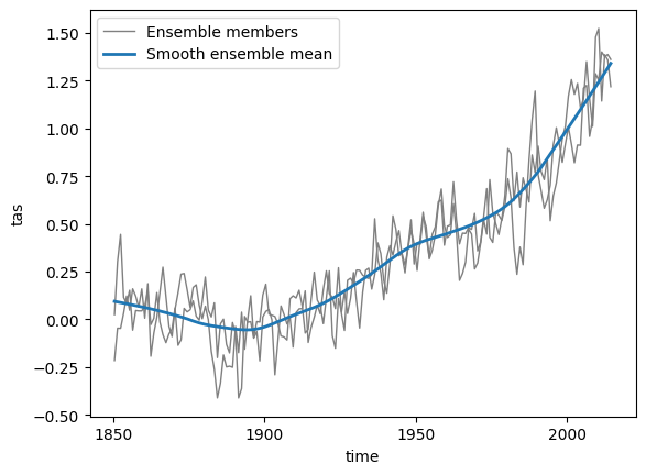
Fit the parameter of the volcanic contributions only on the historical smoothed data of all ensemble members available. The future scenarios do not have volcanic contributions.
hist_tas_residuals = tas_globmean["historical"] - tas_globmean_smoothed["historical"]

# fit volcanic influence
volcanic_params = mesmer.volc.fit_volcanic_influence(hist_tas_residuals.tas)

volcanic_params.aod
Downloading file 'obs/tau.line_2012.12.txt' from 'https://github.com/MESMER-group/mesmer/raw/v1.0.0rc1/data/obs/tau.line_2012.12.txt' to '/home/docs/.cache/mesmer/v1.0.0rc1'.
<xarray.DataArray 'aod' ()> Size: 8B
array(-1.75209374)
- -1.752
array(-1.75209374)
Superimpose the volcanic influence on the historical time series. Because the historical data is treated as its own scenario, we encounter discontinuities at the boundary between historical and future period. However, this is not relevant for the fitting of the parameters hereafter.
# superimpose the volcanic forcing on historical data
tas_globmean_smoothed["historical"] = mesmer.volc.superimpose_volcanic_influence(
    tas_globmean_smoothed["historical"],
    volcanic_params,
)
# plot global mean time series
f, ax = plt.subplots()

# plot unsmoothed global means
tas_globmean["historical"].tas.plot.line(
    ax=ax, lw=1, x="time", color="0.5", add_legend=False
)
tas_globmean["ssp126"].tas.plot.line(
    ax=ax, lw=1, x="time", color="#6baed6", add_legend=False
)
tas_globmean["ssp585"].tas.plot.line(
    ax=ax, lw=1, x="time", color="#fc9272", add_legend=False
)

# plot smoothed global means including volcanic influence for historical
tas_globmean_smoothed["historical"].tas.plot.line(
    ax=ax, lw=1.5, x="time", color="0.1", label="historical"
)
tas_globmean_smoothed["ssp126"].tas.plot.line(
    ax=ax, lw=1.5, x="time", color="#08519c", label="ssp126"
)
tas_globmean_smoothed["ssp585"].tas.plot.line(
    ax=ax, lw=1.5, x="time", color="#de2d26", label="ssp585"
)

# histend = tas_globmean["historical"].time.isel(time=-1).item()
# ax.axvline(histend, color="0.4")
ax.axhline(0, color="0.1", lw=0.5)

ax.set_title("")
plt.legend(loc="upper left")
<matplotlib.legend.Legend at 0x7c92170913a0>
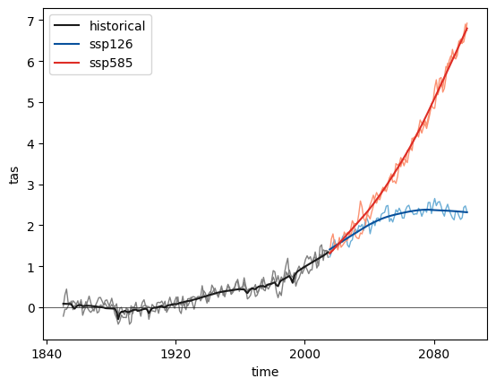
Calculate residuals (w.r.t. smoothed ts) i.e. remove the smoothed global mean, including the volcanic influence from the anomalies.
tas_globmean_resids = tas_globmean - tas_globmean_smoothed
# rename to tas_resids
tas_globmean_resids = mesmer.datatree.map_over_datasets(
    lambda ds: ds.rename({"tas": "tas_resids"}), tas_globmean_resids
)
# plot residuals
h0, *_ = tas_globmean_resids["historical"].tas_resids.plot.line(
    x="time", color="0.5", lw=1, add_legend=False
)
h1, *_ = tas_globmean_resids["ssp126"].tas_resids.plot.line(
    x="time", color="#08519c", lw=1, add_legend=False
)
h2, *_ = tas_globmean_resids["ssp585"].tas_resids.plot.line(
    x="time", color="#de2d26", lw=1, add_legend=False
)

plt.title("Residuals")
plt.axhline(0, lw=1, color="0.1")

plt.legend([h0, h1, h2], ["historical", "ssp126", "ssp585"])
<matplotlib.legend.Legend at 0x7c92160d6fc0>
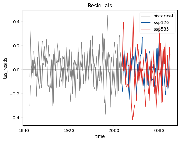
Global variability#
In this step we want to fit an AR process for estimating global variability, taking in the residual global mean temperature as follows:
We first estimate the order of the AR process and then fit the parameters. Internally, we fit the parameters for each member and then average first over the parameters of each scenario and then over all scenarios to arrive at a single set of parameters.
ar_order = mesmer.stats.select_ar_order_scen_ens(
    tas_globmean_resids, dim="time", ens_dim="member", maxlag=12, ic="bic"
)

global_ar_params = mesmer.stats.fit_auto_regression_scen_ens(
    tas_globmean_resids, dim="time", ens_dim="member", lags=ar_order
)

global_ar_params = global_ar_params.drop_vars("nobs")
global_ar_params
<xarray.Dataset> Size: 32B
Dimensions:    (lags: 1)
Coordinates:
  * lags       (lags) int64 8B 1
Data variables:
    intercept  float64 8B 0.00323
    coeffs     (lags) float64 8B 0.4462
variance float64 8B 0.01379- lags: 1
- lags(lags)int641
array([1])
- intercept()float640.00323
array(0.00322968)
- coeffs(lags)float640.4462
array([0.44617039])
- variance()float640.01379
array(0.01379473)
- lagsPandasIndex
PandasIndex(Index([1], dtype='int64', name='lags'))
Local forced response#
Now we need to estimate how the global trend translates into a local forced response. This is done using a linear regression of the global trend and the global variability as predictors:
\(T_{s,t}^{resp} = \beta_s^{int} + \beta_s^{trend} \cdot T_t^{glob,\,trend} + \beta_s^{var} \cdot T_t^{glob,\,var}\)
To this end, we stack all values (members, scenarios) into a single dataset, the only important thing is that predictor and predicted values stay together.
Before computing the coefficients we need to prepare the local temperature data:
Mask out ocean grid points (where the land fraction is larger than
THRESHOLD_LAND)Mask out Antarctica
Convert the data from a 2D lat-lon grid to a 1D grid by stacking it and removing all gridcells that were previously masked out.
Before stacking, we extract the original grid. We need to save this together with the parameters to later be able to reconstruct the original grid from the gridpoints.
# extract original grid
grid_orig = tas_anom["historical"].ds[["lat", "lon"]]
def mask_and_stack(dt, threshold_land):
    dt = mesmer.mask.mask_ocean_fraction(dt, threshold_land)
    dt = mesmer.mask.mask_antarctica(dt)
    dt = mesmer.grid.stack_lat_lon(dt)
    return dt


# mask and stack the data
tas_stacked = mask_and_stack(tas_anom, THRESHOLD_LAND)
Downloading data from 'https://naturalearth.s3.amazonaws.com/5.0.0/110m_physical/ne_110m_land.zip' to file '/home/docs/.cache/regionmask/natural_earth/v5.0.0/ne_110m_land.zip'.
SHA256 hash of downloaded file: 1926c621afd6ac67c3f36639bb1236134a48d82226dc675d3e3df53d02d2a3de
Use this value as the 'known_hash' argument of 'pooch.retrieve' to ensure that the file hasn't changed if it is downloaded again in the future.
Unzipping contents of '/home/docs/.cache/regionmask/natural_earth/v5.0.0/ne_110m_land.zip' to '/home/docs/.cache/regionmask/natural_earth/v5.0.0/ne_110m_land'
tas_stacked["ssp585"].tas.isel(member=1).plot()
<matplotlib.collections.QuadMesh at 0x7c92193b5820>
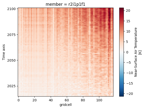
We have now converted the 3D field (with dimensions lat, lon, and time) to a 2D field (with dimensions gridcell and time).
We create a new DataTree from all predictors - here the smoothed global mean and it’s residuals. We could add more predictors, e.g. the squared temperatures or the ocean heat uptake:
predictors = mesmer.datatree.merge([tas_globmean_smoothed, tas_globmean_resids])

target = tas_stacked.copy()
In the linear regression, we want to weight the values of the different scenarios equally, i.e. we do not want scenarios with more members (here ssp585) be overrepresented in the linear regression parameters. Thus, we generate weights that weigh each value by the number of members in their scenario, so \(w_{scen, mem, ts} = 1 / n\_mem_{scen}\). We do currently not take different number of timesteps (historical vs. scenario) into account:
# create weights
weights = mesmer.weighted.equal_scenario_weights_from_datatree(tas_stacked)
weights
<xarray.DatasetView> Size: 0B
Dimensions:  ()
Data variables:
*empty*<xarray.DatasetView> Size: 4kB Dimensions: (time: 165, member: 2) Coordinates: * time (time) object 1kB 1850-07-01 06:00:00 ... 2014-07-01 06:00:00 * member (member) <U8 64B 'r1i1p1f1' 'r2i1p1f1' Data variables: weights (time, member) float64 3kB 0.5 0.5 0.5 0.5 0.5 ... 0.5 0.5 0.5 0.5historical- time: 165
- member: 2
- time(time)object1850-07-01 06:00:00 ... 2014-07-...
- standard_name :
- time
- long_name :
- Time axis
- bounds :
- time_bnds
- axis :
- T
array([cftime.DatetimeGregorian(1850, 7, 1, 6, 0, 0, 0, has_year_zero=False), cftime.DatetimeGregorian(1851, 7, 1, 6, 0, 0, 0, has_year_zero=False), cftime.DatetimeGregorian(1852, 7, 1, 6, 0, 0, 0, has_year_zero=False), cftime.DatetimeGregorian(1853, 7, 1, 6, 0, 0, 0, has_year_zero=False), cftime.DatetimeGregorian(1854, 7, 1, 6, 0, 0, 0, has_year_zero=False), cftime.DatetimeGregorian(1855, 7, 1, 6, 0, 0, 0, has_year_zero=False), cftime.DatetimeGregorian(1856, 7, 1, 6, 0, 0, 0, has_year_zero=False), cftime.DatetimeGregorian(1857, 7, 1, 6, 0, 0, 0, has_year_zero=False), cftime.DatetimeGregorian(1858, 7, 1, 6, 0, 0, 0, has_year_zero=False), cftime.DatetimeGregorian(1859, 7, 1, 6, 0, 0, 0, has_year_zero=False), cftime.DatetimeGregorian(1860, 7, 1, 6, 0, 0, 0, has_year_zero=False), cftime.DatetimeGregorian(1861, 7, 1, 6, 0, 0, 0, has_year_zero=False), cftime.DatetimeGregorian(1862, 7, 1, 6, 0, 0, 0, has_year_zero=False), cftime.DatetimeGregorian(1863, 7, 1, 6, 0, 0, 0, has_year_zero=False), cftime.DatetimeGregorian(1864, 7, 1, 6, 0, 0, 0, has_year_zero=False), cftime.DatetimeGregorian(1865, 7, 1, 6, 0, 0, 0, has_year_zero=False), cftime.DatetimeGregorian(1866, 7, 1, 6, 0, 0, 0, has_year_zero=False), cftime.DatetimeGregorian(1867, 7, 1, 6, 0, 0, 0, has_year_zero=False), cftime.DatetimeGregorian(1868, 7, 1, 6, 0, 0, 0, has_year_zero=False), cftime.DatetimeGregorian(1869, 7, 1, 6, 0, 0, 0, has_year_zero=False), cftime.DatetimeGregorian(1870, 7, 1, 6, 0, 0, 0, has_year_zero=False), cftime.DatetimeGregorian(1871, 7, 1, 6, 0, 0, 0, has_year_zero=False), cftime.DatetimeGregorian(1872, 7, 1, 6, 0, 0, 0, has_year_zero=False), cftime.DatetimeGregorian(1873, 7, 1, 6, 0, 0, 0, has_year_zero=False), cftime.DatetimeGregorian(1874, 7, 1, 6, 0, 0, 0, has_year_zero=False), cftime.DatetimeGregorian(1875, 7, 1, 6, 0, 0, 0, has_year_zero=False), cftime.DatetimeGregorian(1876, 7, 1, 6, 0, 0, 0, has_year_zero=False), cftime.DatetimeGregorian(1877, 7, 1, 6, 0, 0, 0, has_year_zero=False), cftime.DatetimeGregorian(1878, 7, 1, 6, 0, 0, 0, has_year_zero=False), cftime.DatetimeGregorian(1879, 7, 1, 6, 0, 0, 0, has_year_zero=False), cftime.DatetimeGregorian(1880, 7, 1, 6, 0, 0, 0, has_year_zero=False), cftime.DatetimeGregorian(1881, 7, 1, 6, 0, 0, 0, has_year_zero=False), cftime.DatetimeGregorian(1882, 7, 1, 6, 0, 0, 0, has_year_zero=False), cftime.DatetimeGregorian(1883, 7, 1, 6, 0, 0, 0, has_year_zero=False), cftime.DatetimeGregorian(1884, 7, 1, 6, 0, 0, 0, has_year_zero=False), cftime.DatetimeGregorian(1885, 7, 1, 6, 0, 0, 0, has_year_zero=False), cftime.DatetimeGregorian(1886, 7, 1, 6, 0, 0, 0, has_year_zero=False), cftime.DatetimeGregorian(1887, 7, 1, 6, 0, 0, 0, has_year_zero=False), cftime.DatetimeGregorian(1888, 7, 1, 6, 0, 0, 0, has_year_zero=False), cftime.DatetimeGregorian(1889, 7, 1, 6, 0, 0, 0, has_year_zero=False), cftime.DatetimeGregorian(1890, 7, 1, 6, 0, 0, 0, has_year_zero=False), cftime.DatetimeGregorian(1891, 7, 1, 6, 0, 0, 0, has_year_zero=False), cftime.DatetimeGregorian(1892, 7, 1, 6, 0, 0, 0, has_year_zero=False), cftime.DatetimeGregorian(1893, 7, 1, 6, 0, 0, 0, has_year_zero=False), cftime.DatetimeGregorian(1894, 7, 1, 6, 0, 0, 0, has_year_zero=False), cftime.DatetimeGregorian(1895, 7, 1, 6, 0, 0, 0, has_year_zero=False), cftime.DatetimeGregorian(1896, 7, 1, 6, 0, 0, 0, has_year_zero=False), cftime.DatetimeGregorian(1897, 7, 1, 6, 0, 0, 0, has_year_zero=False), cftime.DatetimeGregorian(1898, 7, 1, 6, 0, 0, 0, has_year_zero=False), cftime.DatetimeGregorian(1899, 7, 1, 6, 0, 0, 0, has_year_zero=False), cftime.DatetimeGregorian(1900, 7, 1, 6, 0, 0, 0, has_year_zero=False), cftime.DatetimeGregorian(1901, 7, 1, 6, 0, 0, 0, has_year_zero=False), cftime.DatetimeGregorian(1902, 7, 1, 6, 0, 0, 0, has_year_zero=False), cftime.DatetimeGregorian(1903, 7, 1, 6, 0, 0, 0, has_year_zero=False), cftime.DatetimeGregorian(1904, 7, 1, 6, 0, 0, 0, has_year_zero=False), cftime.DatetimeGregorian(1905, 7, 1, 6, 0, 0, 0, has_year_zero=False), cftime.DatetimeGregorian(1906, 7, 1, 6, 0, 0, 0, has_year_zero=False), cftime.DatetimeGregorian(1907, 7, 1, 6, 0, 0, 0, has_year_zero=False), cftime.DatetimeGregorian(1908, 7, 1, 6, 0, 0, 0, has_year_zero=False), cftime.DatetimeGregorian(1909, 7, 1, 6, 0, 0, 0, has_year_zero=False), cftime.DatetimeGregorian(1910, 7, 1, 6, 0, 0, 0, has_year_zero=False), cftime.DatetimeGregorian(1911, 7, 1, 6, 0, 0, 0, has_year_zero=False), cftime.DatetimeGregorian(1912, 7, 1, 6, 0, 0, 0, has_year_zero=False), cftime.DatetimeGregorian(1913, 7, 1, 6, 0, 0, 0, has_year_zero=False), cftime.DatetimeGregorian(1914, 7, 1, 6, 0, 0, 0, has_year_zero=False), cftime.DatetimeGregorian(1915, 7, 1, 6, 0, 0, 0, has_year_zero=False), cftime.DatetimeGregorian(1916, 7, 1, 6, 0, 0, 0, has_year_zero=False), cftime.DatetimeGregorian(1917, 7, 1, 6, 0, 0, 0, has_year_zero=False), cftime.DatetimeGregorian(1918, 7, 1, 6, 0, 0, 0, has_year_zero=False), cftime.DatetimeGregorian(1919, 7, 1, 6, 0, 0, 0, has_year_zero=False), cftime.DatetimeGregorian(1920, 7, 1, 6, 0, 0, 0, has_year_zero=False), cftime.DatetimeGregorian(1921, 7, 1, 6, 0, 0, 0, has_year_zero=False), cftime.DatetimeGregorian(1922, 7, 1, 6, 0, 0, 0, has_year_zero=False), cftime.DatetimeGregorian(1923, 7, 1, 6, 0, 0, 0, has_year_zero=False), cftime.DatetimeGregorian(1924, 7, 1, 6, 0, 0, 0, has_year_zero=False), cftime.DatetimeGregorian(1925, 7, 1, 6, 0, 0, 0, has_year_zero=False), cftime.DatetimeGregorian(1926, 7, 1, 6, 0, 0, 0, has_year_zero=False), cftime.DatetimeGregorian(1927, 7, 1, 6, 0, 0, 0, has_year_zero=False), cftime.DatetimeGregorian(1928, 7, 1, 6, 0, 0, 0, has_year_zero=False), cftime.DatetimeGregorian(1929, 7, 1, 6, 0, 0, 0, has_year_zero=False), cftime.DatetimeGregorian(1930, 7, 1, 6, 0, 0, 0, has_year_zero=False), cftime.DatetimeGregorian(1931, 7, 1, 6, 0, 0, 0, has_year_zero=False), cftime.DatetimeGregorian(1932, 7, 1, 6, 0, 0, 0, has_year_zero=False), cftime.DatetimeGregorian(1933, 7, 1, 6, 0, 0, 0, has_year_zero=False), cftime.DatetimeGregorian(1934, 7, 1, 6, 0, 0, 0, has_year_zero=False), cftime.DatetimeGregorian(1935, 7, 1, 6, 0, 0, 0, has_year_zero=False), cftime.DatetimeGregorian(1936, 7, 1, 6, 0, 0, 0, has_year_zero=False), cftime.DatetimeGregorian(1937, 7, 1, 6, 0, 0, 0, has_year_zero=False), cftime.DatetimeGregorian(1938, 7, 1, 6, 0, 0, 0, has_year_zero=False), cftime.DatetimeGregorian(1939, 7, 1, 6, 0, 0, 0, has_year_zero=False), cftime.DatetimeGregorian(1940, 7, 1, 6, 0, 0, 0, has_year_zero=False), cftime.DatetimeGregorian(1941, 7, 1, 6, 0, 0, 0, has_year_zero=False), cftime.DatetimeGregorian(1942, 7, 1, 6, 0, 0, 0, has_year_zero=False), cftime.DatetimeGregorian(1943, 7, 1, 6, 0, 0, 0, has_year_zero=False), cftime.DatetimeGregorian(1944, 7, 1, 6, 0, 0, 0, has_year_zero=False), cftime.DatetimeGregorian(1945, 7, 1, 6, 0, 0, 0, has_year_zero=False), cftime.DatetimeGregorian(1946, 7, 1, 6, 0, 0, 0, has_year_zero=False), cftime.DatetimeGregorian(1947, 7, 1, 6, 0, 0, 0, has_year_zero=False), cftime.DatetimeGregorian(1948, 7, 1, 6, 0, 0, 0, has_year_zero=False), cftime.DatetimeGregorian(1949, 7, 1, 6, 0, 0, 0, has_year_zero=False), cftime.DatetimeGregorian(1950, 7, 1, 6, 0, 0, 0, has_year_zero=False), cftime.DatetimeGregorian(1951, 7, 1, 6, 0, 0, 0, has_year_zero=False), cftime.DatetimeGregorian(1952, 7, 1, 6, 0, 0, 0, has_year_zero=False), cftime.DatetimeGregorian(1953, 7, 1, 6, 0, 0, 0, has_year_zero=False), cftime.DatetimeGregorian(1954, 7, 1, 6, 0, 0, 0, has_year_zero=False), cftime.DatetimeGregorian(1955, 7, 1, 6, 0, 0, 0, has_year_zero=False), cftime.DatetimeGregorian(1956, 7, 1, 6, 0, 0, 0, has_year_zero=False), cftime.DatetimeGregorian(1957, 7, 1, 6, 0, 0, 0, has_year_zero=False), cftime.DatetimeGregorian(1958, 7, 1, 6, 0, 0, 0, has_year_zero=False), cftime.DatetimeGregorian(1959, 7, 1, 6, 0, 0, 0, has_year_zero=False), cftime.DatetimeGregorian(1960, 7, 1, 6, 0, 0, 0, has_year_zero=False), cftime.DatetimeGregorian(1961, 7, 1, 6, 0, 0, 0, has_year_zero=False), cftime.DatetimeGregorian(1962, 7, 1, 6, 0, 0, 0, has_year_zero=False), cftime.DatetimeGregorian(1963, 7, 1, 6, 0, 0, 0, has_year_zero=False), cftime.DatetimeGregorian(1964, 7, 1, 6, 0, 0, 0, has_year_zero=False), cftime.DatetimeGregorian(1965, 7, 1, 6, 0, 0, 0, has_year_zero=False), cftime.DatetimeGregorian(1966, 7, 1, 6, 0, 0, 0, has_year_zero=False), cftime.DatetimeGregorian(1967, 7, 1, 6, 0, 0, 0, has_year_zero=False), cftime.DatetimeGregorian(1968, 7, 1, 6, 0, 0, 0, has_year_zero=False), cftime.DatetimeGregorian(1969, 7, 1, 6, 0, 0, 0, has_year_zero=False), cftime.DatetimeGregorian(1970, 7, 1, 6, 0, 0, 0, has_year_zero=False), cftime.DatetimeGregorian(1971, 7, 1, 6, 0, 0, 0, has_year_zero=False), cftime.DatetimeGregorian(1972, 7, 1, 6, 0, 0, 0, has_year_zero=False), cftime.DatetimeGregorian(1973, 7, 1, 6, 0, 0, 0, has_year_zero=False), cftime.DatetimeGregorian(1974, 7, 1, 6, 0, 0, 0, has_year_zero=False), cftime.DatetimeGregorian(1975, 7, 1, 6, 0, 0, 0, has_year_zero=False), cftime.DatetimeGregorian(1976, 7, 1, 6, 0, 0, 0, has_year_zero=False), cftime.DatetimeGregorian(1977, 7, 1, 6, 0, 0, 0, has_year_zero=False), cftime.DatetimeGregorian(1978, 7, 1, 6, 0, 0, 0, has_year_zero=False), cftime.DatetimeGregorian(1979, 7, 1, 6, 0, 0, 0, has_year_zero=False), cftime.DatetimeGregorian(1980, 7, 1, 6, 0, 0, 0, has_year_zero=False), cftime.DatetimeGregorian(1981, 7, 1, 6, 0, 0, 0, has_year_zero=False), cftime.DatetimeGregorian(1982, 7, 1, 6, 0, 0, 0, has_year_zero=False), cftime.DatetimeGregorian(1983, 7, 1, 6, 0, 0, 0, has_year_zero=False), cftime.DatetimeGregorian(1984, 7, 1, 6, 0, 0, 0, has_year_zero=False), cftime.DatetimeGregorian(1985, 7, 1, 6, 0, 0, 0, has_year_zero=False), cftime.DatetimeGregorian(1986, 7, 1, 6, 0, 0, 0, has_year_zero=False), cftime.DatetimeGregorian(1987, 7, 1, 6, 0, 0, 0, has_year_zero=False), cftime.DatetimeGregorian(1988, 7, 1, 6, 0, 0, 0, has_year_zero=False), cftime.DatetimeGregorian(1989, 7, 1, 6, 0, 0, 0, has_year_zero=False), cftime.DatetimeGregorian(1990, 7, 1, 6, 0, 0, 0, has_year_zero=False), cftime.DatetimeGregorian(1991, 7, 1, 6, 0, 0, 0, has_year_zero=False), cftime.DatetimeGregorian(1992, 7, 1, 6, 0, 0, 0, has_year_zero=False), cftime.DatetimeGregorian(1993, 7, 1, 6, 0, 0, 0, has_year_zero=False), cftime.DatetimeGregorian(1994, 7, 1, 6, 0, 0, 0, has_year_zero=False), cftime.DatetimeGregorian(1995, 7, 1, 6, 0, 0, 0, has_year_zero=False), cftime.DatetimeGregorian(1996, 7, 1, 6, 0, 0, 0, has_year_zero=False), cftime.DatetimeGregorian(1997, 7, 1, 6, 0, 0, 0, has_year_zero=False), cftime.DatetimeGregorian(1998, 7, 1, 6, 0, 0, 0, has_year_zero=False), cftime.DatetimeGregorian(1999, 7, 1, 6, 0, 0, 0, has_year_zero=False), cftime.DatetimeGregorian(2000, 7, 1, 6, 0, 0, 0, has_year_zero=False), cftime.DatetimeGregorian(2001, 7, 1, 6, 0, 0, 0, has_year_zero=False), cftime.DatetimeGregorian(2002, 7, 1, 6, 0, 0, 0, has_year_zero=False), cftime.DatetimeGregorian(2003, 7, 1, 6, 0, 0, 0, has_year_zero=False), cftime.DatetimeGregorian(2004, 7, 1, 6, 0, 0, 0, has_year_zero=False), cftime.DatetimeGregorian(2005, 7, 1, 6, 0, 0, 0, has_year_zero=False), cftime.DatetimeGregorian(2006, 7, 1, 6, 0, 0, 0, has_year_zero=False), cftime.DatetimeGregorian(2007, 7, 1, 6, 0, 0, 0, has_year_zero=False), cftime.DatetimeGregorian(2008, 7, 1, 6, 0, 0, 0, has_year_zero=False), cftime.DatetimeGregorian(2009, 7, 1, 6, 0, 0, 0, has_year_zero=False), cftime.DatetimeGregorian(2010, 7, 1, 6, 0, 0, 0, has_year_zero=False), cftime.DatetimeGregorian(2011, 7, 1, 6, 0, 0, 0, has_year_zero=False), cftime.DatetimeGregorian(2012, 7, 1, 6, 0, 0, 0, has_year_zero=False), cftime.DatetimeGregorian(2013, 7, 1, 6, 0, 0, 0, has_year_zero=False), cftime.DatetimeGregorian(2014, 7, 1, 6, 0, 0, 0, has_year_zero=False)], dtype=object) - member(member)<U8'r1i1p1f1' 'r2i1p1f1'
array(['r1i1p1f1', 'r2i1p1f1'], dtype='<U8')
- weights(time, member)float640.5 0.5 0.5 0.5 ... 0.5 0.5 0.5 0.5
array([[0.5, 0.5],
       [0.5, 0.5],
       [0.5, 0.5],
       [0.5, 0.5],
       [0.5, 0.5],
       [0.5, 0.5],
       [0.5, 0.5],
       [0.5, 0.5],
       [0.5, 0.5],
       [0.5, 0.5],
       [0.5, 0.5],
       [0.5, 0.5],
       [0.5, 0.5],
       [0.5, 0.5],
       [0.5, 0.5],
       [0.5, 0.5],
       [0.5, 0.5],
       [0.5, 0.5],
       [0.5, 0.5],
       [0.5, 0.5],
...
       [0.5, 0.5],
       [0.5, 0.5],
       [0.5, 0.5],
       [0.5, 0.5],
       [0.5, 0.5],
       [0.5, 0.5],
       [0.5, 0.5],
       [0.5, 0.5],
       [0.5, 0.5],
       [0.5, 0.5],
       [0.5, 0.5],
       [0.5, 0.5],
       [0.5, 0.5],
       [0.5, 0.5],
       [0.5, 0.5],
       [0.5, 0.5],
       [0.5, 0.5],
       [0.5, 0.5],
       [0.5, 0.5],
       [0.5, 0.5]])
<xarray.DatasetView> Size: 1kB Dimensions: (time: 86, member: 1) Coordinates: * time (time) object 688B 2015-07-01 06:00:00 ... 2100-07-01 06:00:00 * member (member) <U8 32B 'r1i1p1f1' Data variables: weights (time, member) float64 688B 1.0 1.0 1.0 1.0 1.0 ... 1.0 1.0 1.0 1.0ssp126- time: 86
- member: 1
- time(time)object2015-07-01 06:00:00 ... 2100-07-...
- standard_name :
- time
- long_name :
- Time axis
- bounds :
- time_bnds
- axis :
- T
array([cftime.DatetimeGregorian(2015, 7, 1, 6, 0, 0, 0, has_year_zero=False), cftime.DatetimeGregorian(2016, 7, 1, 6, 0, 0, 0, has_year_zero=False), cftime.DatetimeGregorian(2017, 7, 1, 6, 0, 0, 0, has_year_zero=False), cftime.DatetimeGregorian(2018, 7, 1, 6, 0, 0, 0, has_year_zero=False), cftime.DatetimeGregorian(2019, 7, 1, 6, 0, 0, 0, has_year_zero=False), cftime.DatetimeGregorian(2020, 7, 1, 6, 0, 0, 0, has_year_zero=False), cftime.DatetimeGregorian(2021, 7, 1, 6, 0, 0, 0, has_year_zero=False), cftime.DatetimeGregorian(2022, 7, 1, 6, 0, 0, 0, has_year_zero=False), cftime.DatetimeGregorian(2023, 7, 1, 6, 0, 0, 0, has_year_zero=False), cftime.DatetimeGregorian(2024, 7, 1, 6, 0, 0, 0, has_year_zero=False), cftime.DatetimeGregorian(2025, 7, 1, 6, 0, 0, 0, has_year_zero=False), cftime.DatetimeGregorian(2026, 7, 1, 6, 0, 0, 0, has_year_zero=False), cftime.DatetimeGregorian(2027, 7, 1, 6, 0, 0, 0, has_year_zero=False), cftime.DatetimeGregorian(2028, 7, 1, 6, 0, 0, 0, has_year_zero=False), cftime.DatetimeGregorian(2029, 7, 1, 6, 0, 0, 0, has_year_zero=False), cftime.DatetimeGregorian(2030, 7, 1, 6, 0, 0, 0, has_year_zero=False), cftime.DatetimeGregorian(2031, 7, 1, 6, 0, 0, 0, has_year_zero=False), cftime.DatetimeGregorian(2032, 7, 1, 6, 0, 0, 0, has_year_zero=False), cftime.DatetimeGregorian(2033, 7, 1, 6, 0, 0, 0, has_year_zero=False), cftime.DatetimeGregorian(2034, 7, 1, 6, 0, 0, 0, has_year_zero=False), cftime.DatetimeGregorian(2035, 7, 1, 6, 0, 0, 0, has_year_zero=False), cftime.DatetimeGregorian(2036, 7, 1, 6, 0, 0, 0, has_year_zero=False), cftime.DatetimeGregorian(2037, 7, 1, 6, 0, 0, 0, has_year_zero=False), cftime.DatetimeGregorian(2038, 7, 1, 6, 0, 0, 0, has_year_zero=False), cftime.DatetimeGregorian(2039, 7, 1, 6, 0, 0, 0, has_year_zero=False), cftime.DatetimeGregorian(2040, 7, 1, 6, 0, 0, 0, has_year_zero=False), cftime.DatetimeGregorian(2041, 7, 1, 6, 0, 0, 0, has_year_zero=False), cftime.DatetimeGregorian(2042, 7, 1, 6, 0, 0, 0, has_year_zero=False), cftime.DatetimeGregorian(2043, 7, 1, 6, 0, 0, 0, has_year_zero=False), cftime.DatetimeGregorian(2044, 7, 1, 6, 0, 0, 0, has_year_zero=False), cftime.DatetimeGregorian(2045, 7, 1, 6, 0, 0, 0, has_year_zero=False), cftime.DatetimeGregorian(2046, 7, 1, 6, 0, 0, 0, has_year_zero=False), cftime.DatetimeGregorian(2047, 7, 1, 6, 0, 0, 0, has_year_zero=False), cftime.DatetimeGregorian(2048, 7, 1, 6, 0, 0, 0, has_year_zero=False), cftime.DatetimeGregorian(2049, 7, 1, 6, 0, 0, 0, has_year_zero=False), cftime.DatetimeGregorian(2050, 7, 1, 6, 0, 0, 0, has_year_zero=False), cftime.DatetimeGregorian(2051, 7, 1, 6, 0, 0, 0, has_year_zero=False), cftime.DatetimeGregorian(2052, 7, 1, 6, 0, 0, 0, has_year_zero=False), cftime.DatetimeGregorian(2053, 7, 1, 6, 0, 0, 0, has_year_zero=False), cftime.DatetimeGregorian(2054, 7, 1, 6, 0, 0, 0, has_year_zero=False), cftime.DatetimeGregorian(2055, 7, 1, 6, 0, 0, 0, has_year_zero=False), cftime.DatetimeGregorian(2056, 7, 1, 6, 0, 0, 0, has_year_zero=False), cftime.DatetimeGregorian(2057, 7, 1, 6, 0, 0, 0, has_year_zero=False), cftime.DatetimeGregorian(2058, 7, 1, 6, 0, 0, 0, has_year_zero=False), cftime.DatetimeGregorian(2059, 7, 1, 6, 0, 0, 0, has_year_zero=False), cftime.DatetimeGregorian(2060, 7, 1, 6, 0, 0, 0, has_year_zero=False), cftime.DatetimeGregorian(2061, 7, 1, 6, 0, 0, 0, has_year_zero=False), cftime.DatetimeGregorian(2062, 7, 1, 6, 0, 0, 0, has_year_zero=False), cftime.DatetimeGregorian(2063, 7, 1, 6, 0, 0, 0, has_year_zero=False), cftime.DatetimeGregorian(2064, 7, 1, 6, 0, 0, 0, has_year_zero=False), cftime.DatetimeGregorian(2065, 7, 1, 6, 0, 0, 0, has_year_zero=False), cftime.DatetimeGregorian(2066, 7, 1, 6, 0, 0, 0, has_year_zero=False), cftime.DatetimeGregorian(2067, 7, 1, 6, 0, 0, 0, has_year_zero=False), cftime.DatetimeGregorian(2068, 7, 1, 6, 0, 0, 0, has_year_zero=False), cftime.DatetimeGregorian(2069, 7, 1, 6, 0, 0, 0, has_year_zero=False), cftime.DatetimeGregorian(2070, 7, 1, 6, 0, 0, 0, has_year_zero=False), cftime.DatetimeGregorian(2071, 7, 1, 6, 0, 0, 0, has_year_zero=False), cftime.DatetimeGregorian(2072, 7, 1, 6, 0, 0, 0, has_year_zero=False), cftime.DatetimeGregorian(2073, 7, 1, 6, 0, 0, 0, has_year_zero=False), cftime.DatetimeGregorian(2074, 7, 1, 6, 0, 0, 0, has_year_zero=False), cftime.DatetimeGregorian(2075, 7, 1, 6, 0, 0, 0, has_year_zero=False), cftime.DatetimeGregorian(2076, 7, 1, 6, 0, 0, 0, has_year_zero=False), cftime.DatetimeGregorian(2077, 7, 1, 6, 0, 0, 0, has_year_zero=False), cftime.DatetimeGregorian(2078, 7, 1, 6, 0, 0, 0, has_year_zero=False), cftime.DatetimeGregorian(2079, 7, 1, 6, 0, 0, 0, has_year_zero=False), cftime.DatetimeGregorian(2080, 7, 1, 6, 0, 0, 0, has_year_zero=False), cftime.DatetimeGregorian(2081, 7, 1, 6, 0, 0, 0, has_year_zero=False), cftime.DatetimeGregorian(2082, 7, 1, 6, 0, 0, 0, has_year_zero=False), cftime.DatetimeGregorian(2083, 7, 1, 6, 0, 0, 0, has_year_zero=False), cftime.DatetimeGregorian(2084, 7, 1, 6, 0, 0, 0, has_year_zero=False), cftime.DatetimeGregorian(2085, 7, 1, 6, 0, 0, 0, has_year_zero=False), cftime.DatetimeGregorian(2086, 7, 1, 6, 0, 0, 0, has_year_zero=False), cftime.DatetimeGregorian(2087, 7, 1, 6, 0, 0, 0, has_year_zero=False), cftime.DatetimeGregorian(2088, 7, 1, 6, 0, 0, 0, has_year_zero=False), cftime.DatetimeGregorian(2089, 7, 1, 6, 0, 0, 0, has_year_zero=False), cftime.DatetimeGregorian(2090, 7, 1, 6, 0, 0, 0, has_year_zero=False), cftime.DatetimeGregorian(2091, 7, 1, 6, 0, 0, 0, has_year_zero=False), cftime.DatetimeGregorian(2092, 7, 1, 6, 0, 0, 0, has_year_zero=False), cftime.DatetimeGregorian(2093, 7, 1, 6, 0, 0, 0, has_year_zero=False), cftime.DatetimeGregorian(2094, 7, 1, 6, 0, 0, 0, has_year_zero=False), cftime.DatetimeGregorian(2095, 7, 1, 6, 0, 0, 0, has_year_zero=False), cftime.DatetimeGregorian(2096, 7, 1, 6, 0, 0, 0, has_year_zero=False), cftime.DatetimeGregorian(2097, 7, 1, 6, 0, 0, 0, has_year_zero=False), cftime.DatetimeGregorian(2098, 7, 1, 6, 0, 0, 0, has_year_zero=False), cftime.DatetimeGregorian(2099, 7, 1, 6, 0, 0, 0, has_year_zero=False), cftime.DatetimeGregorian(2100, 7, 1, 6, 0, 0, 0, has_year_zero=False)], dtype=object) - member(member)<U8'r1i1p1f1'
array(['r1i1p1f1'], dtype='<U8')
- weights(time, member)float641.0 1.0 1.0 1.0 ... 1.0 1.0 1.0 1.0
array([[1.],
       [1.],
       [1.],
       [1.],
       [1.],
       [1.],
       [1.],
       [1.],
       [1.],
       [1.],
       [1.],
       [1.],
       [1.],
       [1.],
       [1.],
       [1.],
       [1.],
       [1.],
       [1.],
       [1.],
...
       [1.],
       [1.],
       [1.],
       [1.],
       [1.],
       [1.],
       [1.],
       [1.],
       [1.],
       [1.],
       [1.],
       [1.],
       [1.],
       [1.],
       [1.],
       [1.],
       [1.],
       [1.],
       [1.],
       [1.]])
<xarray.DatasetView> Size: 2kB Dimensions: (time: 86, member: 2) Coordinates: * time (time) object 688B 2015-07-01 06:00:00 ... 2100-07-01 06:00:00 * member (member) <U8 64B 'r1i1p1f1' 'r2i1p1f1' Data variables: weights (time, member) float64 1kB 0.5 0.5 0.5 0.5 0.5 ... 0.5 0.5 0.5 0.5ssp585- time: 86
- member: 2
- time(time)object2015-07-01 06:00:00 ... 2100-07-...
- standard_name :
- time
- long_name :
- Time axis
- bounds :
- time_bnds
- axis :
- T
array([cftime.DatetimeGregorian(2015, 7, 1, 6, 0, 0, 0, has_year_zero=False), cftime.DatetimeGregorian(2016, 7, 1, 6, 0, 0, 0, has_year_zero=False), cftime.DatetimeGregorian(2017, 7, 1, 6, 0, 0, 0, has_year_zero=False), cftime.DatetimeGregorian(2018, 7, 1, 6, 0, 0, 0, has_year_zero=False), cftime.DatetimeGregorian(2019, 7, 1, 6, 0, 0, 0, has_year_zero=False), cftime.DatetimeGregorian(2020, 7, 1, 6, 0, 0, 0, has_year_zero=False), cftime.DatetimeGregorian(2021, 7, 1, 6, 0, 0, 0, has_year_zero=False), cftime.DatetimeGregorian(2022, 7, 1, 6, 0, 0, 0, has_year_zero=False), cftime.DatetimeGregorian(2023, 7, 1, 6, 0, 0, 0, has_year_zero=False), cftime.DatetimeGregorian(2024, 7, 1, 6, 0, 0, 0, has_year_zero=False), cftime.DatetimeGregorian(2025, 7, 1, 6, 0, 0, 0, has_year_zero=False), cftime.DatetimeGregorian(2026, 7, 1, 6, 0, 0, 0, has_year_zero=False), cftime.DatetimeGregorian(2027, 7, 1, 6, 0, 0, 0, has_year_zero=False), cftime.DatetimeGregorian(2028, 7, 1, 6, 0, 0, 0, has_year_zero=False), cftime.DatetimeGregorian(2029, 7, 1, 6, 0, 0, 0, has_year_zero=False), cftime.DatetimeGregorian(2030, 7, 1, 6, 0, 0, 0, has_year_zero=False), cftime.DatetimeGregorian(2031, 7, 1, 6, 0, 0, 0, has_year_zero=False), cftime.DatetimeGregorian(2032, 7, 1, 6, 0, 0, 0, has_year_zero=False), cftime.DatetimeGregorian(2033, 7, 1, 6, 0, 0, 0, has_year_zero=False), cftime.DatetimeGregorian(2034, 7, 1, 6, 0, 0, 0, has_year_zero=False), cftime.DatetimeGregorian(2035, 7, 1, 6, 0, 0, 0, has_year_zero=False), cftime.DatetimeGregorian(2036, 7, 1, 6, 0, 0, 0, has_year_zero=False), cftime.DatetimeGregorian(2037, 7, 1, 6, 0, 0, 0, has_year_zero=False), cftime.DatetimeGregorian(2038, 7, 1, 6, 0, 0, 0, has_year_zero=False), cftime.DatetimeGregorian(2039, 7, 1, 6, 0, 0, 0, has_year_zero=False), cftime.DatetimeGregorian(2040, 7, 1, 6, 0, 0, 0, has_year_zero=False), cftime.DatetimeGregorian(2041, 7, 1, 6, 0, 0, 0, has_year_zero=False), cftime.DatetimeGregorian(2042, 7, 1, 6, 0, 0, 0, has_year_zero=False), cftime.DatetimeGregorian(2043, 7, 1, 6, 0, 0, 0, has_year_zero=False), cftime.DatetimeGregorian(2044, 7, 1, 6, 0, 0, 0, has_year_zero=False), cftime.DatetimeGregorian(2045, 7, 1, 6, 0, 0, 0, has_year_zero=False), cftime.DatetimeGregorian(2046, 7, 1, 6, 0, 0, 0, has_year_zero=False), cftime.DatetimeGregorian(2047, 7, 1, 6, 0, 0, 0, has_year_zero=False), cftime.DatetimeGregorian(2048, 7, 1, 6, 0, 0, 0, has_year_zero=False), cftime.DatetimeGregorian(2049, 7, 1, 6, 0, 0, 0, has_year_zero=False), cftime.DatetimeGregorian(2050, 7, 1, 6, 0, 0, 0, has_year_zero=False), cftime.DatetimeGregorian(2051, 7, 1, 6, 0, 0, 0, has_year_zero=False), cftime.DatetimeGregorian(2052, 7, 1, 6, 0, 0, 0, has_year_zero=False), cftime.DatetimeGregorian(2053, 7, 1, 6, 0, 0, 0, has_year_zero=False), cftime.DatetimeGregorian(2054, 7, 1, 6, 0, 0, 0, has_year_zero=False), cftime.DatetimeGregorian(2055, 7, 1, 6, 0, 0, 0, has_year_zero=False), cftime.DatetimeGregorian(2056, 7, 1, 6, 0, 0, 0, has_year_zero=False), cftime.DatetimeGregorian(2057, 7, 1, 6, 0, 0, 0, has_year_zero=False), cftime.DatetimeGregorian(2058, 7, 1, 6, 0, 0, 0, has_year_zero=False), cftime.DatetimeGregorian(2059, 7, 1, 6, 0, 0, 0, has_year_zero=False), cftime.DatetimeGregorian(2060, 7, 1, 6, 0, 0, 0, has_year_zero=False), cftime.DatetimeGregorian(2061, 7, 1, 6, 0, 0, 0, has_year_zero=False), cftime.DatetimeGregorian(2062, 7, 1, 6, 0, 0, 0, has_year_zero=False), cftime.DatetimeGregorian(2063, 7, 1, 6, 0, 0, 0, has_year_zero=False), cftime.DatetimeGregorian(2064, 7, 1, 6, 0, 0, 0, has_year_zero=False), cftime.DatetimeGregorian(2065, 7, 1, 6, 0, 0, 0, has_year_zero=False), cftime.DatetimeGregorian(2066, 7, 1, 6, 0, 0, 0, has_year_zero=False), cftime.DatetimeGregorian(2067, 7, 1, 6, 0, 0, 0, has_year_zero=False), cftime.DatetimeGregorian(2068, 7, 1, 6, 0, 0, 0, has_year_zero=False), cftime.DatetimeGregorian(2069, 7, 1, 6, 0, 0, 0, has_year_zero=False), cftime.DatetimeGregorian(2070, 7, 1, 6, 0, 0, 0, has_year_zero=False), cftime.DatetimeGregorian(2071, 7, 1, 6, 0, 0, 0, has_year_zero=False), cftime.DatetimeGregorian(2072, 7, 1, 6, 0, 0, 0, has_year_zero=False), cftime.DatetimeGregorian(2073, 7, 1, 6, 0, 0, 0, has_year_zero=False), cftime.DatetimeGregorian(2074, 7, 1, 6, 0, 0, 0, has_year_zero=False), cftime.DatetimeGregorian(2075, 7, 1, 6, 0, 0, 0, has_year_zero=False), cftime.DatetimeGregorian(2076, 7, 1, 6, 0, 0, 0, has_year_zero=False), cftime.DatetimeGregorian(2077, 7, 1, 6, 0, 0, 0, has_year_zero=False), cftime.DatetimeGregorian(2078, 7, 1, 6, 0, 0, 0, has_year_zero=False), cftime.DatetimeGregorian(2079, 7, 1, 6, 0, 0, 0, has_year_zero=False), cftime.DatetimeGregorian(2080, 7, 1, 6, 0, 0, 0, has_year_zero=False), cftime.DatetimeGregorian(2081, 7, 1, 6, 0, 0, 0, has_year_zero=False), cftime.DatetimeGregorian(2082, 7, 1, 6, 0, 0, 0, has_year_zero=False), cftime.DatetimeGregorian(2083, 7, 1, 6, 0, 0, 0, has_year_zero=False), cftime.DatetimeGregorian(2084, 7, 1, 6, 0, 0, 0, has_year_zero=False), cftime.DatetimeGregorian(2085, 7, 1, 6, 0, 0, 0, has_year_zero=False), cftime.DatetimeGregorian(2086, 7, 1, 6, 0, 0, 0, has_year_zero=False), cftime.DatetimeGregorian(2087, 7, 1, 6, 0, 0, 0, has_year_zero=False), cftime.DatetimeGregorian(2088, 7, 1, 6, 0, 0, 0, has_year_zero=False), cftime.DatetimeGregorian(2089, 7, 1, 6, 0, 0, 0, has_year_zero=False), cftime.DatetimeGregorian(2090, 7, 1, 6, 0, 0, 0, has_year_zero=False), cftime.DatetimeGregorian(2091, 7, 1, 6, 0, 0, 0, has_year_zero=False), cftime.DatetimeGregorian(2092, 7, 1, 6, 0, 0, 0, has_year_zero=False), cftime.DatetimeGregorian(2093, 7, 1, 6, 0, 0, 0, has_year_zero=False), cftime.DatetimeGregorian(2094, 7, 1, 6, 0, 0, 0, has_year_zero=False), cftime.DatetimeGregorian(2095, 7, 1, 6, 0, 0, 0, has_year_zero=False), cftime.DatetimeGregorian(2096, 7, 1, 6, 0, 0, 0, has_year_zero=False), cftime.DatetimeGregorian(2097, 7, 1, 6, 0, 0, 0, has_year_zero=False), cftime.DatetimeGregorian(2098, 7, 1, 6, 0, 0, 0, has_year_zero=False), cftime.DatetimeGregorian(2099, 7, 1, 6, 0, 0, 0, has_year_zero=False), cftime.DatetimeGregorian(2100, 7, 1, 6, 0, 0, 0, has_year_zero=False)], dtype=object) - member(member)<U8'r1i1p1f1' 'r2i1p1f1'
array(['r1i1p1f1', 'r2i1p1f1'], dtype='<U8')
- weights(time, member)float640.5 0.5 0.5 0.5 ... 0.5 0.5 0.5 0.5
array([[0.5, 0.5],
       [0.5, 0.5],
       [0.5, 0.5],
       [0.5, 0.5],
       [0.5, 0.5],
       [0.5, 0.5],
       [0.5, 0.5],
       [0.5, 0.5],
       [0.5, 0.5],
       [0.5, 0.5],
       [0.5, 0.5],
       [0.5, 0.5],
       [0.5, 0.5],
       [0.5, 0.5],
       [0.5, 0.5],
       [0.5, 0.5],
       [0.5, 0.5],
       [0.5, 0.5],
       [0.5, 0.5],
       [0.5, 0.5],
...
       [0.5, 0.5],
       [0.5, 0.5],
       [0.5, 0.5],
       [0.5, 0.5],
       [0.5, 0.5],
       [0.5, 0.5],
       [0.5, 0.5],
       [0.5, 0.5],
       [0.5, 0.5],
       [0.5, 0.5],
       [0.5, 0.5],
       [0.5, 0.5],
       [0.5, 0.5],
       [0.5, 0.5],
       [0.5, 0.5],
       [0.5, 0.5],
       [0.5, 0.5],
       [0.5, 0.5],
       [0.5, 0.5],
       [0.5, 0.5]])
We pool the different scenarios, ensemble members and timesteps into one sample dimension (containing time, member, and scenario as coordinates) for the linear regression. We want one DataArray per predictor and the target such that each sample of the predictor variables aligns with the corresponding sample of the target:
predictors_pooled, target_pooled, weights_pooled = (
    mesmer.datatree.broadcast_and_pool_scen_ens(predictors, target, weights)
)

target_pooled
<xarray.Dataset> Size: 585kB
Dimensions:   (gridcell: 118, sample: 588)
Coordinates:
    scenario  (sample) object 5kB 'historical' 'historical' ... 'ssp585'
    time      (sample) object 5kB 1850-07-01 06:00:00 ... 2100-07-01 06:00:00
    member    (sample) <U8 19kB 'r1i1p1f1' 'r1i1p1f1' ... 'r2i1p1f1' 'r2i1p1f1'
    lat       (gridcell) float64 944B -49.5 -40.5 -31.5 -31.5 ... 76.5 76.5 76.5
    lon       (gridcell) float64 944B 288.0 288.0 18.0 ... 306.0 324.0 342.0
Dimensions without coordinates: gridcell, sample
Data variables:
    tas       (sample, gridcell) float64 555kB -0.1548 -0.1209 ... 13.42 16.16
Attributes: (12/56)
    CDI:                       Climate Data Interface version 1.9.9 (https://...
    source:                    IPSL-CM6A-LR (2017):  atmos: LMDZ (NPv6, N96; ...
    institution:               Institut Pierre Simon Laplace, Paris 75252, Fr...
    Conventions:               CF-1.7 CMIP-6.2
    history:                   Thu Mar 18 19:05:09 2021: cdo remapbil,r20x20 ...
    creation_date:             2018-07-11T07:36:34Z
    ...                        ...
    realization_index:         1
    NCO:                       "4.6.0"
    cmip6-ng:                  \ncontact = cmip6-archive@env.ethz.ch\ndescrip...
    original_file_names:       /net/atmos/data/cmip6/historical/Amon/tas/IPSL...
    original_file_hash_codes:  7264c228560257b32d44dcc611d92976da7214af7e8795...
CDO: Climate Data Operators version 1.9.9 (https://...- gridcell: 118
- sample: 588
- scenario(sample)object'historical' ... 'ssp585'
array(['historical', 'historical', 'historical', 'historical', 'historical', 'historical', 'historical', 'historical', 'historical', 'historical', 'historical', 'historical', 'historical', 'historical', 'historical', 'historical', 'historical', 'historical', 'historical', 'historical', 'historical', 'historical', 'historical', 'historical', 'historical', 'historical', 'historical', 'historical', 'historical', 'historical', 'historical', 'historical', 'historical', 'historical', 'historical', 'historical', 'historical', 'historical', 'historical', 'historical', 'historical', 'historical', 'historical', 'historical', 'historical', 'historical', 'historical', 'historical', 'historical', 'historical', 'historical', 'historical', 'historical', 'historical', 'historical', 'historical', 'historical', 'historical', 'historical', 'historical', 'historical', 'historical', 'historical', 'historical', 'historical', 'historical', 'historical', 'historical', 'historical', 'historical', 'historical', 'historical', 'historical', 'historical', 'historical', 'historical', 'historical', 'historical', 'historical', 'historical', ... 'ssp585', 'ssp585', 'ssp585', 'ssp585', 'ssp585', 'ssp585', 'ssp585', 'ssp585', 'ssp585', 'ssp585', 'ssp585', 'ssp585', 'ssp585', 'ssp585', 'ssp585', 'ssp585', 'ssp585', 'ssp585', 'ssp585', 'ssp585', 'ssp585', 'ssp585', 'ssp585', 'ssp585', 'ssp585', 'ssp585', 'ssp585', 'ssp585', 'ssp585', 'ssp585', 'ssp585', 'ssp585', 'ssp585', 'ssp585', 'ssp585', 'ssp585', 'ssp585', 'ssp585', 'ssp585', 'ssp585', 'ssp585', 'ssp585', 'ssp585', 'ssp585', 'ssp585', 'ssp585', 'ssp585', 'ssp585', 'ssp585', 'ssp585', 'ssp585', 'ssp585', 'ssp585', 'ssp585', 'ssp585', 'ssp585', 'ssp585', 'ssp585', 'ssp585', 'ssp585', 'ssp585', 'ssp585', 'ssp585', 'ssp585', 'ssp585', 'ssp585', 'ssp585', 'ssp585', 'ssp585', 'ssp585', 'ssp585', 'ssp585', 'ssp585', 'ssp585', 'ssp585', 'ssp585', 'ssp585', 'ssp585', 'ssp585', 'ssp585', 'ssp585', 'ssp585', 'ssp585', 'ssp585', 'ssp585', 'ssp585', 'ssp585', 'ssp585', 'ssp585', 'ssp585', 'ssp585', 'ssp585', 'ssp585', 'ssp585', 'ssp585', 'ssp585', 'ssp585', 'ssp585', 'ssp585', 'ssp585', 'ssp585', 'ssp585', 'ssp585', 'ssp585', 'ssp585', 'ssp585', 'ssp585', 'ssp585', 'ssp585', 'ssp585', 'ssp585', 'ssp585', 'ssp585', 'ssp585', 'ssp585', 'ssp585'], dtype=object) - time(sample)object1850-07-01 06:00:00 ... 2100-07-...
- standard_name :
- time
- long_name :
- Time axis
- bounds :
- time_bnds
- axis :
- T
array([cftime.DatetimeGregorian(1850, 7, 1, 6, 0, 0, 0, has_year_zero=False), cftime.DatetimeGregorian(1851, 7, 1, 6, 0, 0, 0, has_year_zero=False), cftime.DatetimeGregorian(1852, 7, 1, 6, 0, 0, 0, has_year_zero=False), cftime.DatetimeGregorian(1853, 7, 1, 6, 0, 0, 0, has_year_zero=False), cftime.DatetimeGregorian(1854, 7, 1, 6, 0, 0, 0, has_year_zero=False), cftime.DatetimeGregorian(1855, 7, 1, 6, 0, 0, 0, has_year_zero=False), cftime.DatetimeGregorian(1856, 7, 1, 6, 0, 0, 0, has_year_zero=False), cftime.DatetimeGregorian(1857, 7, 1, 6, 0, 0, 0, has_year_zero=False), cftime.DatetimeGregorian(1858, 7, 1, 6, 0, 0, 0, has_year_zero=False), cftime.DatetimeGregorian(1859, 7, 1, 6, 0, 0, 0, has_year_zero=False), cftime.DatetimeGregorian(1860, 7, 1, 6, 0, 0, 0, has_year_zero=False), cftime.DatetimeGregorian(1861, 7, 1, 6, 0, 0, 0, has_year_zero=False), cftime.DatetimeGregorian(1862, 7, 1, 6, 0, 0, 0, has_year_zero=False), cftime.DatetimeGregorian(1863, 7, 1, 6, 0, 0, 0, has_year_zero=False), cftime.DatetimeGregorian(1864, 7, 1, 6, 0, 0, 0, has_year_zero=False), cftime.DatetimeGregorian(1865, 7, 1, 6, 0, 0, 0, has_year_zero=False), cftime.DatetimeGregorian(1866, 7, 1, 6, 0, 0, 0, has_year_zero=False), cftime.DatetimeGregorian(1867, 7, 1, 6, 0, 0, 0, has_year_zero=False), cftime.DatetimeGregorian(1868, 7, 1, 6, 0, 0, 0, has_year_zero=False), cftime.DatetimeGregorian(1869, 7, 1, 6, 0, 0, 0, has_year_zero=False), ... cftime.DatetimeGregorian(2082, 7, 1, 6, 0, 0, 0, has_year_zero=False), cftime.DatetimeGregorian(2083, 7, 1, 6, 0, 0, 0, has_year_zero=False), cftime.DatetimeGregorian(2084, 7, 1, 6, 0, 0, 0, has_year_zero=False), cftime.DatetimeGregorian(2085, 7, 1, 6, 0, 0, 0, has_year_zero=False), cftime.DatetimeGregorian(2086, 7, 1, 6, 0, 0, 0, has_year_zero=False), cftime.DatetimeGregorian(2087, 7, 1, 6, 0, 0, 0, has_year_zero=False), cftime.DatetimeGregorian(2088, 7, 1, 6, 0, 0, 0, has_year_zero=False), cftime.DatetimeGregorian(2089, 7, 1, 6, 0, 0, 0, has_year_zero=False), cftime.DatetimeGregorian(2090, 7, 1, 6, 0, 0, 0, has_year_zero=False), cftime.DatetimeGregorian(2091, 7, 1, 6, 0, 0, 0, has_year_zero=False), cftime.DatetimeGregorian(2092, 7, 1, 6, 0, 0, 0, has_year_zero=False), cftime.DatetimeGregorian(2093, 7, 1, 6, 0, 0, 0, has_year_zero=False), cftime.DatetimeGregorian(2094, 7, 1, 6, 0, 0, 0, has_year_zero=False), cftime.DatetimeGregorian(2095, 7, 1, 6, 0, 0, 0, has_year_zero=False), cftime.DatetimeGregorian(2096, 7, 1, 6, 0, 0, 0, has_year_zero=False), cftime.DatetimeGregorian(2097, 7, 1, 6, 0, 0, 0, has_year_zero=False), cftime.DatetimeGregorian(2098, 7, 1, 6, 0, 0, 0, has_year_zero=False), cftime.DatetimeGregorian(2099, 7, 1, 6, 0, 0, 0, has_year_zero=False), cftime.DatetimeGregorian(2100, 7, 1, 6, 0, 0, 0, has_year_zero=False)], dtype=object) - member(sample)<U8'r1i1p1f1' ... 'r2i1p1f1'
array(['r1i1p1f1', 'r1i1p1f1', 'r1i1p1f1', 'r1i1p1f1', 'r1i1p1f1', 'r1i1p1f1', 'r1i1p1f1', 'r1i1p1f1', 'r1i1p1f1', 'r1i1p1f1', 'r1i1p1f1', 'r1i1p1f1', 'r1i1p1f1', 'r1i1p1f1', 'r1i1p1f1', 'r1i1p1f1', 'r1i1p1f1', 'r1i1p1f1', 'r1i1p1f1', 'r1i1p1f1', 'r1i1p1f1', 'r1i1p1f1', 'r1i1p1f1', 'r1i1p1f1', 'r1i1p1f1', 'r1i1p1f1', 'r1i1p1f1', 'r1i1p1f1', 'r1i1p1f1', 'r1i1p1f1', 'r1i1p1f1', 'r1i1p1f1', 'r1i1p1f1', 'r1i1p1f1', 'r1i1p1f1', 'r1i1p1f1', 'r1i1p1f1', 'r1i1p1f1', 'r1i1p1f1', 'r1i1p1f1', 'r1i1p1f1', 'r1i1p1f1', 'r1i1p1f1', 'r1i1p1f1', 'r1i1p1f1', 'r1i1p1f1', 'r1i1p1f1', 'r1i1p1f1', 'r1i1p1f1', 'r1i1p1f1', 'r1i1p1f1', 'r1i1p1f1', 'r1i1p1f1', 'r1i1p1f1', 'r1i1p1f1', 'r1i1p1f1', 'r1i1p1f1', 'r1i1p1f1', 'r1i1p1f1', 'r1i1p1f1', 'r1i1p1f1', 'r1i1p1f1', 'r1i1p1f1', 'r1i1p1f1', 'r1i1p1f1', 'r1i1p1f1', 'r1i1p1f1', 'r1i1p1f1', 'r1i1p1f1', 'r1i1p1f1', 'r1i1p1f1', 'r1i1p1f1', 'r1i1p1f1', 'r1i1p1f1', 'r1i1p1f1', 'r1i1p1f1', 'r1i1p1f1', 'r1i1p1f1', 'r1i1p1f1', 'r1i1p1f1', 'r1i1p1f1', 'r1i1p1f1', 'r1i1p1f1', 'r1i1p1f1', 'r1i1p1f1', 'r1i1p1f1', 'r1i1p1f1', 'r1i1p1f1', 'r1i1p1f1', 'r1i1p1f1', 'r1i1p1f1', 'r1i1p1f1', 'r1i1p1f1', 'r1i1p1f1', 'r1i1p1f1', 'r1i1p1f1', 'r1i1p1f1', 'r1i1p1f1', 'r1i1p1f1', 'r1i1p1f1', ... 'r1i1p1f1', 'r1i1p1f1', 'r1i1p1f1', 'r1i1p1f1', 'r1i1p1f1', 'r1i1p1f1', 'r1i1p1f1', 'r1i1p1f1', 'r1i1p1f1', 'r1i1p1f1', 'r1i1p1f1', 'r1i1p1f1', 'r2i1p1f1', 'r2i1p1f1', 'r2i1p1f1', 'r2i1p1f1', 'r2i1p1f1', 'r2i1p1f1', 'r2i1p1f1', 'r2i1p1f1', 'r2i1p1f1', 'r2i1p1f1', 'r2i1p1f1', 'r2i1p1f1', 'r2i1p1f1', 'r2i1p1f1', 'r2i1p1f1', 'r2i1p1f1', 'r2i1p1f1', 'r2i1p1f1', 'r2i1p1f1', 'r2i1p1f1', 'r2i1p1f1', 'r2i1p1f1', 'r2i1p1f1', 'r2i1p1f1', 'r2i1p1f1', 'r2i1p1f1', 'r2i1p1f1', 'r2i1p1f1', 'r2i1p1f1', 'r2i1p1f1', 'r2i1p1f1', 'r2i1p1f1', 'r2i1p1f1', 'r2i1p1f1', 'r2i1p1f1', 'r2i1p1f1', 'r2i1p1f1', 'r2i1p1f1', 'r2i1p1f1', 'r2i1p1f1', 'r2i1p1f1', 'r2i1p1f1', 'r2i1p1f1', 'r2i1p1f1', 'r2i1p1f1', 'r2i1p1f1', 'r2i1p1f1', 'r2i1p1f1', 'r2i1p1f1', 'r2i1p1f1', 'r2i1p1f1', 'r2i1p1f1', 'r2i1p1f1', 'r2i1p1f1', 'r2i1p1f1', 'r2i1p1f1', 'r2i1p1f1', 'r2i1p1f1', 'r2i1p1f1', 'r2i1p1f1', 'r2i1p1f1', 'r2i1p1f1', 'r2i1p1f1', 'r2i1p1f1', 'r2i1p1f1', 'r2i1p1f1', 'r2i1p1f1', 'r2i1p1f1', 'r2i1p1f1', 'r2i1p1f1', 'r2i1p1f1', 'r2i1p1f1', 'r2i1p1f1', 'r2i1p1f1', 'r2i1p1f1', 'r2i1p1f1', 'r2i1p1f1', 'r2i1p1f1', 'r2i1p1f1', 'r2i1p1f1', 'r2i1p1f1', 'r2i1p1f1', 'r2i1p1f1', 'r2i1p1f1', 'r2i1p1f1', 'r2i1p1f1'], dtype='<U8') - lat(gridcell)float64-49.5 -40.5 -31.5 ... 76.5 76.5
- standard_name :
- latitude
- long_name :
- latitude
- units :
- degrees_north
- axis :
- Y
array([-49.5, -40.5, -31.5, -31.5, -31.5, -31.5, -31.5, -22.5, -22.5, -22.5, -22.5, -22.5, -22.5, -13.5, -13.5, -13.5, -13.5, -13.5, -13.5, -4.5, -4.5, -4.5, -4.5, -4.5, -4.5, 4.5, 4.5, 4.5, 4.5, 4.5, 13.5, 13.5, 13.5, 13.5, 13.5, 13.5, 22.5, 22.5, 22.5, 22.5, 22.5, 22.5, 22.5, 22.5, 22.5, 31.5, 31.5, 31.5, 31.5, 31.5, 31.5, 31.5, 31.5, 31.5, 40.5, 40.5, 40.5, 40.5, 40.5, 40.5, 40.5, 40.5, 40.5, 40.5, 40.5, 40.5, 49.5, 49.5, 49.5, 49.5, 49.5, 49.5, 49.5, 49.5, 49.5, 49.5, 49.5, 49.5, 58.5, 58.5, 58.5, 58.5, 58.5, 58.5, 58.5, 58.5, 58.5, 58.5, 58.5, 58.5, 58.5, 58.5, 58.5, 67.5, 67.5, 67.5, 67.5, 67.5, 67.5, 67.5, 67.5, 67.5, 67.5, 67.5, 67.5, 67.5, 67.5, 67.5, 67.5, 67.5, 67.5, 76.5, 76.5, 76.5, 76.5, 76.5, 76.5, 76.5]) - lon(gridcell)float64288.0 288.0 18.0 ... 324.0 342.0
- standard_name :
- longitude
- long_name :
- longitude
- units :
- degrees_east
- axis :
- X
array([288., 288.,  18., 126., 144., 288., 306.,  18.,  36., 126., 144.,
       288., 306.,  18.,  36., 126., 288., 306., 324.,  18.,  36., 144.,
       288., 306., 324.,   0.,  18.,  36., 288., 306.,   0.,  18.,  36.,
       108., 270., 342.,   0.,  18.,  36.,  54.,  72.,  90., 108., 252.,
       342.,   0.,  18.,  36.,  54.,  72.,  90., 108., 252., 270.,   0.,
        18.,  36.,  54.,  72.,  90., 108., 126., 234., 252., 270., 288.,
         0.,  18.,  36.,  54.,  72.,  90., 108., 126., 234., 252., 270.,
       288.,  18.,  36.,  54.,  72.,  90., 108., 126., 144., 162., 198.,
       216., 234., 252., 270., 288.,  18.,  36.,  54.,  72.,  90., 108.,
       126., 144., 162., 180., 198., 216., 234., 252., 270., 288., 306.,
       324.,  90., 108., 270., 288., 306., 324., 342.])
- tas(sample, gridcell)float64-0.1548 -0.1209 ... 13.42 16.16
- standard_name :
- air_temperature
- long_name :
- Near-Surface Air Temperature
- units :
- K
- online_operation :
- average
- cell_methods :
- area: time: mean
- interval_operation :
- 900 s
- interval_write :
- 1 month
- description :
- Near-Surface Air Temperature
- history :
- none
- cell_measures :
- area: areacella
array([[-1.54786040e-01, -1.20911864e-01,  4.64801549e-02, ...,
        -1.22614391e+00, -1.16283881e+00, -1.25134319e+00],
       [-2.17608828e-01, -6.01335162e-02,  4.72598980e-02, ...,
        -1.95907467e+00, -2.01640579e+00, -1.85223656e-01],
       [-8.16561317e-01, -6.74846367e-01, -1.44391614e-01, ...,
        -2.58084976e-02, -7.56439646e-01,  5.53803683e-03],
       ...,
       [ 4.66250973e+00,  5.77272776e+00,  4.59209366e+00, ...,
         9.57440258e+00,  1.02341516e+01,  1.52850628e+01],
       [ 4.81733847e+00,  5.41056953e+00,  4.66859501e+00, ...,
         8.74611172e+00,  9.99273916e+00,  1.56117686e+01],
       [ 4.44475123e+00,  5.34127186e+00,  5.12633660e+00, ...,
         1.18474082e+01,  1.34167613e+01,  1.61559676e+01]],
      shape=(588, 118))
- CDI :
- Climate Data Interface version 1.9.9 (https://mpimet.mpg.de/cdi)
- source :
- IPSL-CM6A-LR (2017): atmos: LMDZ (NPv6, N96; 144 x 143 longitude/latitude; 79 levels; top level 40000 m) land: ORCHIDEE (v2.0, Water/Carbon/Energy mode) ocean: NEMO-OPA (eORCA1.3, tripolar primarily 1deg; 362 x 332 longitude/latitude; 75 levels; top grid cell 0-2 m) ocnBgchem: NEMO-PISCES seaIce: NEMO-LIM3
- institution :
- Institut Pierre Simon Laplace, Paris 75252, France
- Conventions :
- CF-1.7 CMIP-6.2
- history :
- Thu Mar 18 19:05:09 2021: cdo remapbil,r20x20 tests/test-data/first-run-test/cmip6-ng//tas/ann/g025/tas_ann_IPSL-CM6A-LR_historical_r1i1p1f1_g025.nc tas_ann_IPSL-CM6A-LR_historical_r1i1p1f1_g025.nc Thu Dec 19 16:26:00 2019: cdo -O -b F64 -remapcon2,../grids/g025.txt /cmip6/Next_Generation.v2/tas/ann/native/tas_ann_IPSL-CM6A-LR_historical_r1i1p1f1_native.nc /cmip6/Next_Generation.v2/tas/ann/g025/tas_ann_IPSL-CM6A-LR_historical_r1i1p1f1_g025.nc Thu Dec 19 16:25:59 2019: cdo -O -b F64 -yearmonmean /cmip6/Next_Generation.v2/tas/mon/native/tas_mon_IPSL-CM6A-LR_historical_r1i1p1f1_native.nc /cmip6/Next_Generation.v2/tas/ann/native/tas_ann_IPSL-CM6A-LR_historical_r1i1p1f1_native.nc Sat Dec 1 12:16:58 2018: ncatted -O -a realization_index,global,m,i,1 /ccc/work/cont003/cmip6/cmip6/onhold/CM61-LR-histEXT-03.1910/files+ext/tas_Amon_IPSL-CM6A-LR_historical_r1i1p1f1_gr_185001-201412.nc Sat Dec 1 12:10:43 2018: ncatted -O -a realization_index,global,m,i,1 /ccc/work/cont003/cmip6/cmip6/onhold/CM61-LR-hist-03.1910/files/tas_Amon_IPSL-CM6A-LR_historical_r1i1p1f1_gr_185001-201412.nc Sat Dec 1 11:05:09 2018: ncatted -O -a realization_index,global,m,i,1 /ccc/work/cont003/gencmip6/p86caub/IGCM_OUT/IPSLCM6/PROD/historical/CM61-LR-hist-03.1910/CMIP6/ATM/tas_Amon_IPSL-CM6A-LR_historical_r1i1p1f1_gr_185001-201412.nc Fri Nov 30 16:51:53 2018: ncatted -O -a realization_index,global,m,s,1 /ccc/work/cont003/gencmip6/p86caub/IGCM_OUT/IPSLCM6/PROD/historical/CM61-LR-hist-03.1910/CMIP6/ATM/tas_Amon_IPSL-CM6A-LR_historical_r1i1p1f1_gr_185001-201412.nc Thu Nov 29 16:51:58 2018: ncatted -O -a variant_label,global,m,c,r1i1p1f1 /ccc/work/cont003/gencmip6/p86caub/IGCM_OUT/IPSLCM6/PROD/historical/CM61-LR-hist-03.1910/CMIP6/ATM/tas_Amon_IPSL-CM6A-LR_historical_r3i1p1f1_gr_185001-201412.nc Thu Nov 29 16:51:58 2018: ncatted -O -a further_info_url,global,m,c,https://furtherinfo.es-doc.org/CMIP6.IPSL.IPSL-CM6A-LR.historical.none.r1i1p1f1 /ccc/work/cont003/gencmip6/p86caub/IGCM_OUT/IPSLCM6/PROD/historical/CM61-LR-hist-03.1910/CMIP6/ATM/tas_Amon_IPSL-CM6A-LR_historical_r3i1p1f1_gr_185001-201412.nc Thu Nov 29 16:51:58 2018: ncatted -O -a name,global,m,c,/ccc/work/cont003/gencmip6/p86caub/IGCM_OUT/IPSLCM6/PROD/historical/CM61-LR-hist-03.1910/CMIP6/ATM/tas_Amon_IPSL-CM6A-LR_historical_r1i1p1f1_gr_%start_date%-%end_date% /ccc/work/cont003/gencmip6/p86caub/IGCM_OUT/IPSLCM6/PROD/historical/CM61-LR-hist-03.1910/CMIP6/ATM/tas_Amon_IPSL-CM6A-LR_historical_r3i1p1f1_gr_185001-201412.nc Mon Sep 3 14:52:55 2018: ncatted -O -a parent_variant_label,global,m,c,r1i1p1f1 tas_Amon_IPSL-CM6A-LR_historical_r3i1p1f1_gr_185001-201412.nc none
- creation_date :
- 2018-07-11T07:36:34Z
- tracking_id :
- hdl:21.14100/285a3a27-0287-4e3b-8232-69ddc89cebef
- description :
- CMIP6 historical
- title :
- IPSL-CM6A-LR model output prepared for CMIP6 / CMIP historical
- activity_id :
- CMIP
- contact :
- ipsl-cmip6@listes.ipsl.fr
- data_specs_version :
- 01.00.21
- dr2xml_version :
- 1.11
- experiment_id :
- historical
- experiment :
- all-forcing simulation of the recent past
- external_variables :
- areacella
- forcing_index :
- 1
- frequency :
- mon
- grid :
- LMDZ grid
- grid_label :
- gr
- nominal_resolution :
- 250 km
- initialization_index :
- 1
- institution_id :
- IPSL
- license :
- CMIP6 model data produced by IPSL is licensed under a Creative Commons Attribution-NonCommercial-ShareAlike 4.0 International License (https://creativecommons.org/licenses). Consult https://pcmdi.llnl.gov/CMIP6/TermsOfUse for terms of use governing CMIP6 output, including citation requirements and proper acknowledgment. Further information about this data, including some limitations, can be found via the further_info_url (recorded as a global attribute in this file) and at https://cmc.ipsl.fr/. The data producers and data providers make no warranty, either express or implied, including, but not limited to, warranties of merchantability and fitness for a particular purpose. All liabilities arising from the supply of the information (including any liability arising in negligence) are excluded to the fullest extent permitted by law.
- mip_era :
- CMIP6
- parent_experiment_id :
- piControl
- parent_mip_era :
- CMIP6
- parent_activity_id :
- CMIP
- parent_source_id :
- IPSL-CM6A-LR
- parent_time_units :
- days since 1850-01-01 00:00:00
- branch_method :
- standard
- branch_time_in_parent :
- 21914.0
- branch_time_in_child :
- 0.0
- physics_index :
- 1
- product :
- model-output
- realm :
- atmos
- source_id :
- IPSL-CM6A-LR
- source_type :
- AOGCM BGC
- sub_experiment_id :
- none
- sub_experiment :
- none
- table_id :
- Amon
- variable_id :
- tas
- EXPID :
- historical
- CMIP6_CV_version :
- cv=6.2.3.5-2-g63b123e
- dr2xml_md5sum :
- f1e40c1fc5d8281f865f72fbf4e38f9d
- model_version :
- 6.1.5
- parent_variant_label :
- r1i1p1f1
- name :
- /ccc/work/cont003/gencmip6/p86caub/IGCM_OUT/IPSLCM6/PROD/historical/CM61-LR-hist-03.1910/CMIP6/ATM/tas_Amon_IPSL-CM6A-LR_historical_r1i1p1f1_gr_%start_date%-%end_date%
- further_info_url :
- https://furtherinfo.es-doc.org/CMIP6.IPSL.IPSL-CM6A-LR.historical.none.r1i1p1f1
- variant_label :
- r1i1p1f1
- realization_index :
- 1
- NCO :
- "4.6.0"
- cmip6-ng :
- contact = cmip6-archive@env.ethz.ch description = ETH Zurich CMIP6 "next generation" (ng) archive. disclaimer = This dataset is provided "as is", without warranty of any kind. fixes = delete time bounds git = 2019-12-17 18:26:09 git@git.iac.ethz.ch:cmip6-ng/cmip6-ng.git: master v1.5-6-g3802cf0 ownership = The ownership of this dataset remains with the original provider unfixed_issues =
- original_file_names :
- /net/atmos/data/cmip6/historical/Amon/tas/IPSL-CM6A-LR/r1i1p1f1/gr/tas_Amon_IPSL-CM6A-LR_historical_r1i1p1f1_gr_185001-201412.nc
- original_file_hash_codes :
- 7264c228560257b32d44dcc611d92976da7214af7e879586a78f969848c8c375
- CDO :
- Climate Data Operators version 1.9.9 (https://mpimet.mpg.de/cdo)
In the linear regression, the predictors for each sample are used for every gridpoint of the target. We can now fit the linear regression:
local_lin_reg = mesmer.stats.LinearRegression()

local_lin_reg.fit(
    predictors=predictors_pooled,
    target=target_pooled.tas,
    dim="sample",
    weights=weights_pooled.weights,
)

local_forced_response_params = local_lin_reg.params
local_forced_response_params
<xarray.Dataset> Size: 38kB
Dimensions:        (gridcell: 118, sample: 588)
Coordinates:
    lat            (gridcell) float64 944B -49.5 -40.5 -31.5 ... 76.5 76.5 76.5
    lon            (gridcell) float64 944B 288.0 288.0 18.0 ... 324.0 342.0
    scenario       (sample) object 5kB 'historical' 'historical' ... 'ssp585'
    time           (sample) object 5kB 1850-07-01 06:00:00 ... 2100-07-01 06:...
    member         (sample) <U8 19kB 'r1i1p1f1' 'r1i1p1f1' ... 'r2i1p1f1'
Dimensions without coordinates: gridcell, sample
Data variables:
    intercept      (gridcell) float64 944B 0.1033 0.02489 ... 0.1346 0.09724
    tas            (gridcell) float64 944B 0.6961 0.8041 0.7246 ... 1.711 2.458
    tas_resids     (gridcell) float64 944B 0.4748 0.4167 0.453 ... 1.675 0.6918
    fit_intercept  bool 1B True
weights (sample) float64 5kB 0.5 0.5 0.5 0.5 0.5 ... 0.5 0.5 0.5 0.5- gridcell: 118
- sample: 588
- lat(gridcell)float64-49.5 -40.5 -31.5 ... 76.5 76.5
- standard_name :
- latitude
- long_name :
- latitude
- units :
- degrees_north
- axis :
- Y
array([-49.5, -40.5, -31.5, -31.5, -31.5, -31.5, -31.5, -22.5, -22.5, -22.5, -22.5, -22.5, -22.5, -13.5, -13.5, -13.5, -13.5, -13.5, -13.5, -4.5, -4.5, -4.5, -4.5, -4.5, -4.5, 4.5, 4.5, 4.5, 4.5, 4.5, 13.5, 13.5, 13.5, 13.5, 13.5, 13.5, 22.5, 22.5, 22.5, 22.5, 22.5, 22.5, 22.5, 22.5, 22.5, 31.5, 31.5, 31.5, 31.5, 31.5, 31.5, 31.5, 31.5, 31.5, 40.5, 40.5, 40.5, 40.5, 40.5, 40.5, 40.5, 40.5, 40.5, 40.5, 40.5, 40.5, 49.5, 49.5, 49.5, 49.5, 49.5, 49.5, 49.5, 49.5, 49.5, 49.5, 49.5, 49.5, 58.5, 58.5, 58.5, 58.5, 58.5, 58.5, 58.5, 58.5, 58.5, 58.5, 58.5, 58.5, 58.5, 58.5, 58.5, 67.5, 67.5, 67.5, 67.5, 67.5, 67.5, 67.5, 67.5, 67.5, 67.5, 67.5, 67.5, 67.5, 67.5, 67.5, 67.5, 67.5, 67.5, 76.5, 76.5, 76.5, 76.5, 76.5, 76.5, 76.5]) - lon(gridcell)float64288.0 288.0 18.0 ... 324.0 342.0
- standard_name :
- longitude
- long_name :
- longitude
- units :
- degrees_east
- axis :
- X
array([288., 288., 18., 126., 144., 288., 306., 18., 36., 126., 144., 288., 306., 18., 36., 126., 288., 306., 324., 18., 36., 144., 288., 306., 324., 0., 18., 36., 288., 306., 0., 18., 36., 108., 270., 342., 0., 18., 36., 54., 72., 90., 108., 252., 342., 0., 18., 36., 54., 72., 90., 108., 252., 270., 0., 18., 36., 54., 72., 90., 108., 126., 234., 252., 270., 288., 0., 18., 36., 54., 72., 90., 108., 126., 234., 252., 270., 288., 18., 36., 54., 72., 90., 108., 126., 144., 162., 198., 216., 234., 252., 270., 288., 18., 36., 54., 72., 90., 108., 126., 144., 162., 180., 198., 216., 234., 252., 270., 288., 306., 324., 90., 108., 270., 288., 306., 324., 342.]) - scenario(sample)object'historical' ... 'ssp585'
array(['historical', 'historical', 'historical', 'historical', 'historical', 'historical', 'historical', 'historical', 'historical', 'historical', 'historical', 'historical', 'historical', 'historical', 'historical', 'historical', 'historical', 'historical', 'historical', 'historical', 'historical', 'historical', 'historical', 'historical', 'historical', 'historical', 'historical', 'historical', 'historical', 'historical', 'historical', 'historical', 'historical', 'historical', 'historical', 'historical', 'historical', 'historical', 'historical', 'historical', 'historical', 'historical', 'historical', 'historical', 'historical', 'historical', 'historical', 'historical', 'historical', 'historical', 'historical', 'historical', 'historical', 'historical', 'historical', 'historical', 'historical', 'historical', 'historical', 'historical', 'historical', 'historical', 'historical', 'historical', 'historical', 'historical', 'historical', 'historical', 'historical', 'historical', 'historical', 'historical', 'historical', 'historical', 'historical', 'historical', 'historical', 'historical', 'historical', 'historical', ... 'ssp585', 'ssp585', 'ssp585', 'ssp585', 'ssp585', 'ssp585', 'ssp585', 'ssp585', 'ssp585', 'ssp585', 'ssp585', 'ssp585', 'ssp585', 'ssp585', 'ssp585', 'ssp585', 'ssp585', 'ssp585', 'ssp585', 'ssp585', 'ssp585', 'ssp585', 'ssp585', 'ssp585', 'ssp585', 'ssp585', 'ssp585', 'ssp585', 'ssp585', 'ssp585', 'ssp585', 'ssp585', 'ssp585', 'ssp585', 'ssp585', 'ssp585', 'ssp585', 'ssp585', 'ssp585', 'ssp585', 'ssp585', 'ssp585', 'ssp585', 'ssp585', 'ssp585', 'ssp585', 'ssp585', 'ssp585', 'ssp585', 'ssp585', 'ssp585', 'ssp585', 'ssp585', 'ssp585', 'ssp585', 'ssp585', 'ssp585', 'ssp585', 'ssp585', 'ssp585', 'ssp585', 'ssp585', 'ssp585', 'ssp585', 'ssp585', 'ssp585', 'ssp585', 'ssp585', 'ssp585', 'ssp585', 'ssp585', 'ssp585', 'ssp585', 'ssp585', 'ssp585', 'ssp585', 'ssp585', 'ssp585', 'ssp585', 'ssp585', 'ssp585', 'ssp585', 'ssp585', 'ssp585', 'ssp585', 'ssp585', 'ssp585', 'ssp585', 'ssp585', 'ssp585', 'ssp585', 'ssp585', 'ssp585', 'ssp585', 'ssp585', 'ssp585', 'ssp585', 'ssp585', 'ssp585', 'ssp585', 'ssp585', 'ssp585', 'ssp585', 'ssp585', 'ssp585', 'ssp585', 'ssp585', 'ssp585', 'ssp585', 'ssp585', 'ssp585', 'ssp585', 'ssp585', 'ssp585', 'ssp585', 'ssp585'], dtype=object) - time(sample)object1850-07-01 06:00:00 ... 2100-07-...
- standard_name :
- time
- long_name :
- Time axis
- bounds :
- time_bnds
- axis :
- T
array([cftime.DatetimeGregorian(1850, 7, 1, 6, 0, 0, 0, has_year_zero=False), cftime.DatetimeGregorian(1851, 7, 1, 6, 0, 0, 0, has_year_zero=False), cftime.DatetimeGregorian(1852, 7, 1, 6, 0, 0, 0, has_year_zero=False), cftime.DatetimeGregorian(1853, 7, 1, 6, 0, 0, 0, has_year_zero=False), cftime.DatetimeGregorian(1854, 7, 1, 6, 0, 0, 0, has_year_zero=False), cftime.DatetimeGregorian(1855, 7, 1, 6, 0, 0, 0, has_year_zero=False), cftime.DatetimeGregorian(1856, 7, 1, 6, 0, 0, 0, has_year_zero=False), cftime.DatetimeGregorian(1857, 7, 1, 6, 0, 0, 0, has_year_zero=False), cftime.DatetimeGregorian(1858, 7, 1, 6, 0, 0, 0, has_year_zero=False), cftime.DatetimeGregorian(1859, 7, 1, 6, 0, 0, 0, has_year_zero=False), cftime.DatetimeGregorian(1860, 7, 1, 6, 0, 0, 0, has_year_zero=False), cftime.DatetimeGregorian(1861, 7, 1, 6, 0, 0, 0, has_year_zero=False), cftime.DatetimeGregorian(1862, 7, 1, 6, 0, 0, 0, has_year_zero=False), cftime.DatetimeGregorian(1863, 7, 1, 6, 0, 0, 0, has_year_zero=False), cftime.DatetimeGregorian(1864, 7, 1, 6, 0, 0, 0, has_year_zero=False), cftime.DatetimeGregorian(1865, 7, 1, 6, 0, 0, 0, has_year_zero=False), cftime.DatetimeGregorian(1866, 7, 1, 6, 0, 0, 0, has_year_zero=False), cftime.DatetimeGregorian(1867, 7, 1, 6, 0, 0, 0, has_year_zero=False), cftime.DatetimeGregorian(1868, 7, 1, 6, 0, 0, 0, has_year_zero=False), cftime.DatetimeGregorian(1869, 7, 1, 6, 0, 0, 0, has_year_zero=False), ... cftime.DatetimeGregorian(2082, 7, 1, 6, 0, 0, 0, has_year_zero=False), cftime.DatetimeGregorian(2083, 7, 1, 6, 0, 0, 0, has_year_zero=False), cftime.DatetimeGregorian(2084, 7, 1, 6, 0, 0, 0, has_year_zero=False), cftime.DatetimeGregorian(2085, 7, 1, 6, 0, 0, 0, has_year_zero=False), cftime.DatetimeGregorian(2086, 7, 1, 6, 0, 0, 0, has_year_zero=False), cftime.DatetimeGregorian(2087, 7, 1, 6, 0, 0, 0, has_year_zero=False), cftime.DatetimeGregorian(2088, 7, 1, 6, 0, 0, 0, has_year_zero=False), cftime.DatetimeGregorian(2089, 7, 1, 6, 0, 0, 0, has_year_zero=False), cftime.DatetimeGregorian(2090, 7, 1, 6, 0, 0, 0, has_year_zero=False), cftime.DatetimeGregorian(2091, 7, 1, 6, 0, 0, 0, has_year_zero=False), cftime.DatetimeGregorian(2092, 7, 1, 6, 0, 0, 0, has_year_zero=False), cftime.DatetimeGregorian(2093, 7, 1, 6, 0, 0, 0, has_year_zero=False), cftime.DatetimeGregorian(2094, 7, 1, 6, 0, 0, 0, has_year_zero=False), cftime.DatetimeGregorian(2095, 7, 1, 6, 0, 0, 0, has_year_zero=False), cftime.DatetimeGregorian(2096, 7, 1, 6, 0, 0, 0, has_year_zero=False), cftime.DatetimeGregorian(2097, 7, 1, 6, 0, 0, 0, has_year_zero=False), cftime.DatetimeGregorian(2098, 7, 1, 6, 0, 0, 0, has_year_zero=False), cftime.DatetimeGregorian(2099, 7, 1, 6, 0, 0, 0, has_year_zero=False), cftime.DatetimeGregorian(2100, 7, 1, 6, 0, 0, 0, has_year_zero=False)], dtype=object) - member(sample)<U8'r1i1p1f1' ... 'r2i1p1f1'
array(['r1i1p1f1', 'r1i1p1f1', 'r1i1p1f1', 'r1i1p1f1', 'r1i1p1f1',
       'r1i1p1f1', 'r1i1p1f1', 'r1i1p1f1', 'r1i1p1f1', 'r1i1p1f1',
       'r1i1p1f1', 'r1i1p1f1', 'r1i1p1f1', 'r1i1p1f1', 'r1i1p1f1',
       'r1i1p1f1', 'r1i1p1f1', 'r1i1p1f1', 'r1i1p1f1', 'r1i1p1f1',
       'r1i1p1f1', 'r1i1p1f1', 'r1i1p1f1', 'r1i1p1f1', 'r1i1p1f1',
       'r1i1p1f1', 'r1i1p1f1', 'r1i1p1f1', 'r1i1p1f1', 'r1i1p1f1',
       'r1i1p1f1', 'r1i1p1f1', 'r1i1p1f1', 'r1i1p1f1', 'r1i1p1f1',
       'r1i1p1f1', 'r1i1p1f1', 'r1i1p1f1', 'r1i1p1f1', 'r1i1p1f1',
       'r1i1p1f1', 'r1i1p1f1', 'r1i1p1f1', 'r1i1p1f1', 'r1i1p1f1',
       'r1i1p1f1', 'r1i1p1f1', 'r1i1p1f1', 'r1i1p1f1', 'r1i1p1f1',
       'r1i1p1f1', 'r1i1p1f1', 'r1i1p1f1', 'r1i1p1f1', 'r1i1p1f1',
       'r1i1p1f1', 'r1i1p1f1', 'r1i1p1f1', 'r1i1p1f1', 'r1i1p1f1',
       'r1i1p1f1', 'r1i1p1f1', 'r1i1p1f1', 'r1i1p1f1', 'r1i1p1f1',
       'r1i1p1f1', 'r1i1p1f1', 'r1i1p1f1', 'r1i1p1f1', 'r1i1p1f1',
       'r1i1p1f1', 'r1i1p1f1', 'r1i1p1f1', 'r1i1p1f1', 'r1i1p1f1',
       'r1i1p1f1', 'r1i1p1f1', 'r1i1p1f1', 'r1i1p1f1', 'r1i1p1f1',
       'r1i1p1f1', 'r1i1p1f1', 'r1i1p1f1', 'r1i1p1f1', 'r1i1p1f1',
       'r1i1p1f1', 'r1i1p1f1', 'r1i1p1f1', 'r1i1p1f1', 'r1i1p1f1',
       'r1i1p1f1', 'r1i1p1f1', 'r1i1p1f1', 'r1i1p1f1', 'r1i1p1f1',
       'r1i1p1f1', 'r1i1p1f1', 'r1i1p1f1', 'r1i1p1f1', 'r1i1p1f1',
...
       'r1i1p1f1', 'r1i1p1f1', 'r1i1p1f1', 'r1i1p1f1', 'r1i1p1f1',
       'r1i1p1f1', 'r1i1p1f1', 'r1i1p1f1', 'r1i1p1f1', 'r1i1p1f1',
       'r1i1p1f1', 'r1i1p1f1', 'r2i1p1f1', 'r2i1p1f1', 'r2i1p1f1',
       'r2i1p1f1', 'r2i1p1f1', 'r2i1p1f1', 'r2i1p1f1', 'r2i1p1f1',
       'r2i1p1f1', 'r2i1p1f1', 'r2i1p1f1', 'r2i1p1f1', 'r2i1p1f1',
       'r2i1p1f1', 'r2i1p1f1', 'r2i1p1f1', 'r2i1p1f1', 'r2i1p1f1',
       'r2i1p1f1', 'r2i1p1f1', 'r2i1p1f1', 'r2i1p1f1', 'r2i1p1f1',
       'r2i1p1f1', 'r2i1p1f1', 'r2i1p1f1', 'r2i1p1f1', 'r2i1p1f1',
       'r2i1p1f1', 'r2i1p1f1', 'r2i1p1f1', 'r2i1p1f1', 'r2i1p1f1',
       'r2i1p1f1', 'r2i1p1f1', 'r2i1p1f1', 'r2i1p1f1', 'r2i1p1f1',
       'r2i1p1f1', 'r2i1p1f1', 'r2i1p1f1', 'r2i1p1f1', 'r2i1p1f1',
       'r2i1p1f1', 'r2i1p1f1', 'r2i1p1f1', 'r2i1p1f1', 'r2i1p1f1',
       'r2i1p1f1', 'r2i1p1f1', 'r2i1p1f1', 'r2i1p1f1', 'r2i1p1f1',
       'r2i1p1f1', 'r2i1p1f1', 'r2i1p1f1', 'r2i1p1f1', 'r2i1p1f1',
       'r2i1p1f1', 'r2i1p1f1', 'r2i1p1f1', 'r2i1p1f1', 'r2i1p1f1',
       'r2i1p1f1', 'r2i1p1f1', 'r2i1p1f1', 'r2i1p1f1', 'r2i1p1f1',
       'r2i1p1f1', 'r2i1p1f1', 'r2i1p1f1', 'r2i1p1f1', 'r2i1p1f1',
       'r2i1p1f1', 'r2i1p1f1', 'r2i1p1f1', 'r2i1p1f1', 'r2i1p1f1',
       'r2i1p1f1', 'r2i1p1f1', 'r2i1p1f1', 'r2i1p1f1', 'r2i1p1f1',
       'r2i1p1f1', 'r2i1p1f1', 'r2i1p1f1'], dtype='<U8')
- intercept(gridcell)float640.1033 0.02489 ... 0.1346 0.09724
array([ 1.03305802e-01, 2.48874211e-02, 6.16362560e-02, -8.08757445e-02, -5.71915306e-02, 6.21317662e-04, -3.18689093e-02, -3.25187816e-02, -3.39015451e-02, -7.23629722e-02, -7.85484956e-02, -2.76973344e-02, -1.04634799e-01, -4.60050228e-02, 1.85787541e-02, 4.60967337e-03, 2.37853678e-02, -7.85015244e-02, 1.51547290e-04, 3.58379259e-02, 2.86075371e-02, 3.21358854e-02, -5.64309533e-02, -1.75421310e-01, 1.84763137e-02, 1.39598924e-02, 1.05257829e-02, 6.34396546e-03, -6.64256880e-02, -3.76125444e-02, 3.64043817e-02, 1.40855565e-02, 4.52741131e-02, -1.64063697e-02, 2.17841725e-03, 2.99767766e-02, 3.87291353e-02, -5.09553904e-02, -5.06425215e-02, 4.28472465e-02, 8.16648748e-03, -7.80702532e-02, -1.55583302e-01, -6.35191729e-02, 1.42011682e-02, 2.73485804e-02, -5.27557266e-02, -1.22170062e-01, 8.86080037e-02, -5.85045549e-02, -3.78488749e-01, -1.59593631e-01, -1.13677060e-01, -1.97162676e-01, -2.23464256e-02, -1.14152134e-01, -1.62225086e-01, -3.29587776e-02, -7.74202345e-02, -1.20612025e-01, -1.42160890e-01, -1.94093425e-01, -9.76460278e-03, -2.61317352e-01, -3.63029041e-01, -8.08509649e-02, 8.42756051e-02, -1.31896636e-01, -3.15729783e-01, -2.58302519e-01, -1.38892740e-01, -1.43449299e-01, -1.76415951e-01, -1.06886128e-01, -1.61778584e-02, -3.02747829e-01, -2.89747697e-01, -2.20780980e-01, 4.91896364e-02, -1.54020725e-01, -2.12610196e-01, -1.07606989e-01, -4.27656119e-02, 1.23934353e-03, 3.44898106e-02, 3.14461966e-01, 1.62251005e-01, 2.22098601e-01, 4.73635006e-02, 7.70700049e-02, -1.09696526e-01, -1.17154598e-01, -1.49621880e-01, 2.20866221e-02, 6.25775436e-02, 1.36718188e-01, 6.28341227e-02, 7.95289476e-02, 9.91303217e-02, 3.32187543e-02, -5.60262505e-02, -1.04463228e-01, -5.11218714e-02, 1.17375266e-01, 1.01626810e-01, 1.18858107e-01, -1.56603848e-01, -1.46693379e-01, -1.39639533e-02, 5.23833424e-01, 2.00921153e-01, 5.29095264e-01, 2.48079391e-01, -3.46915989e-01, 2.97210245e-01, 1.90824486e-01, 1.34645177e-01, 9.72368851e-02]) - tas(gridcell)float640.6961 0.8041 ... 1.711 2.458
array([0.69609472, 0.8041179 , 0.72463869, 0.76108351, 1.06462249, 0.68966087, 0.84450357, 1.23766771, 0.82596301, 1.24343131, 1.11565196, 0.79587143, 1.27306595, 1.15064507, 1.0492373 , 0.88969565, 1.32775511, 1.27442065, 0.70439335, 1.14467191, 1.06454715, 0.8514537 , 1.16851931, 1.27242146, 0.84738192, 0.84428451, 1.12566394, 0.97231164, 1.27855494, 0.97196302, 1.24715983, 1.16655576, 1.06835581, 0.84079922, 1.01031259, 0.71533997, 1.48114715, 1.34893661, 1.15818636, 1.26907572, 1.14357733, 1.02117396, 1.02723501, 0.82218523, 0.59330693, 1.3507362 , 1.03091814, 1.23740521, 1.5241202 , 1.441406 , 1.22982656, 1.37648631, 1.24782259, 1.06585077, 1.18721187, 1.1502249 , 1.26932007, 1.31160496, 1.51140792, 1.53432018, 1.50536061, 1.51016294, 0.87213637, 1.31132034, 1.50413142, 1.29733306, 1.08620351, 1.39761578, 1.52835315, 1.6671394 , 1.70706481, 1.57957745, 1.72229042, 1.74631475, 1.18249798, 1.6023896 , 1.7688413 , 1.73067356, 1.37290001, 1.68764465, 1.82484704, 1.9303548 , 1.95431719, 2.00463922, 2.04303598, 1.85994858, 1.65766368, 1.73124737, 1.15151317, 1.59182251, 1.91055327, 2.25853934, 2.00390681, 1.49639563, 1.65911336, 1.99918719, 2.22202833, 2.13954412, 2.23012867, 2.00534972, 2.08814991, 2.29289935, 2.63164616, 2.46352518, 2.23144829, 2.39277143, 2.56926479, 2.60530478, 2.14636489, 1.9583202 , 1.44862835, 2.66304617, 2.88660743, 3.05547864, 2.51435664, 1.53984411, 1.71126496, 2.45819308]) - tas_resids(gridcell)float640.4748 0.4167 ... 1.675 0.6918
array([ 0.47478608, 0.41666329, 0.45298825, 0.84982175, 1.21421014, 0.96101341, 0.19523735, 1.46871494, 1.16048766, 2.12623562, 2.07984971, 1.96340214, 0.98046373, 1.37113735, 1.23984993, 0.85494073, 2.03169272, 1.62426807, 1.32249414, 1.3333533 , 1.26111274, 0.8999502 , 1.56219128, 2.06016427, 1.16124234, 1.00191192, 1.31948558, 1.6007571 , 2.04508388, 1.61677326, 1.63504307, 1.68696921, 1.54033074, 0.724236 , 1.44177531, 1.0874986 , 1.46008039, 1.50717808, 0.88566926, 1.28947172, 1.56405576, 1.27640054, 1.586846 , 0.12648051, 0.84315424, 1.07602378, 0.83326871, 0.798712 , 0.55549295, 1.28334584, 0.35693974, 1.45046243, -0.2852691 , -0.72291362, 0.45377312, 0.39093639, 0.84931348, 1.10820257, 1.34714883, 0.92695955, 0.54731242, 0.24275463, 1.78949418, 0.21433923, -0.0207576 , 0.2961833 , 0.95413406, 0.76223542, 1.37450352, 1.76240666, 1.6693174 , 0.91427262, 0.62908546, 0.69065714, 2.31150194, 0.94067412, 1.22270432, 1.75633452, 0.94583298, 1.52582489, 1.91385595, 1.99760801, 1.84443502, 1.91968743, 2.01614796, 2.2617098 , 1.22284085, 2.83415955, 2.16053869, 2.85270316, 2.581661 , 1.99568128, 1.93276817, 0.80105094, 1.21056286, 1.84625406, 2.23456342, 2.01534808, 2.27124499, 2.30766904, 2.37975623, 2.09169522, 2.48429128, 3.54504325, 3.29133401, 3.22050607, 2.97034672, 2.05401456, 1.5980677 , 1.1500992 , 1.13304678, 2.94128375, 3.07477054, 2.14082657, 0.79351041, 1.42575058, 1.67479158, 0.69176935]) - fit_intercept()boolTrue
array(True)
- weights(sample)float640.5 0.5 0.5 0.5 ... 0.5 0.5 0.5 0.5
array([0.5, 0.5, 0.5, 0.5, 0.5, 0.5, 0.5, 0.5, 0.5, 0.5, 0.5, 0.5, 0.5,
       0.5, 0.5, 0.5, 0.5, 0.5, 0.5, 0.5, 0.5, 0.5, 0.5, 0.5, 0.5, 0.5,
       0.5, 0.5, 0.5, 0.5, 0.5, 0.5, 0.5, 0.5, 0.5, 0.5, 0.5, 0.5, 0.5,
       0.5, 0.5, 0.5, 0.5, 0.5, 0.5, 0.5, 0.5, 0.5, 0.5, 0.5, 0.5, 0.5,
       0.5, 0.5, 0.5, 0.5, 0.5, 0.5, 0.5, 0.5, 0.5, 0.5, 0.5, 0.5, 0.5,
       0.5, 0.5, 0.5, 0.5, 0.5, 0.5, 0.5, 0.5, 0.5, 0.5, 0.5, 0.5, 0.5,
       0.5, 0.5, 0.5, 0.5, 0.5, 0.5, 0.5, 0.5, 0.5, 0.5, 0.5, 0.5, 0.5,
       0.5, 0.5, 0.5, 0.5, 0.5, 0.5, 0.5, 0.5, 0.5, 0.5, 0.5, 0.5, 0.5,
       0.5, 0.5, 0.5, 0.5, 0.5, 0.5, 0.5, 0.5, 0.5, 0.5, 0.5, 0.5, 0.5,
       0.5, 0.5, 0.5, 0.5, 0.5, 0.5, 0.5, 0.5, 0.5, 0.5, 0.5, 0.5, 0.5,
       0.5, 0.5, 0.5, 0.5, 0.5, 0.5, 0.5, 0.5, 0.5, 0.5, 0.5, 0.5, 0.5,
       0.5, 0.5, 0.5, 0.5, 0.5, 0.5, 0.5, 0.5, 0.5, 0.5, 0.5, 0.5, 0.5,
       0.5, 0.5, 0.5, 0.5, 0.5, 0.5, 0.5, 0.5, 0.5, 0.5, 0.5, 0.5, 0.5,
       0.5, 0.5, 0.5, 0.5, 0.5, 0.5, 0.5, 0.5, 0.5, 0.5, 0.5, 0.5, 0.5,
       0.5, 0.5, 0.5, 0.5, 0.5, 0.5, 0.5, 0.5, 0.5, 0.5, 0.5, 0.5, 0.5,
       0.5, 0.5, 0.5, 0.5, 0.5, 0.5, 0.5, 0.5, 0.5, 0.5, 0.5, 0.5, 0.5,
       0.5, 0.5, 0.5, 0.5, 0.5, 0.5, 0.5, 0.5, 0.5, 0.5, 0.5, 0.5, 0.5,
       0.5, 0.5, 0.5, 0.5, 0.5, 0.5, 0.5, 0.5, 0.5, 0.5, 0.5, 0.5, 0.5,
       0.5, 0.5, 0.5, 0.5, 0.5, 0.5, 0.5, 0.5, 0.5, 0.5, 0.5, 0.5, 0.5,
       0.5, 0.5, 0.5, 0.5, 0.5, 0.5, 0.5, 0.5, 0.5, 0.5, 0.5, 0.5, 0.5,
...
       1. , 1. , 1. , 1. , 1. , 1. , 1. , 1. , 1. , 1. , 1. , 1. , 1. ,
       1. , 1. , 1. , 1. , 1. , 1. , 1. , 1. , 1. , 1. , 1. , 1. , 1. ,
       1. , 1. , 1. , 1. , 1. , 1. , 1. , 1. , 1. , 1. , 1. , 1. , 1. ,
       1. , 1. , 1. , 1. , 1. , 1. , 1. , 1. , 1. , 1. , 1. , 1. , 1. ,
       1. , 1. , 1. , 1. , 1. , 1. , 1. , 1. , 1. , 1. , 1. , 1. , 1. ,
       1. , 1. , 1. , 1. , 1. , 1. , 1. , 1. , 1. , 1. , 1. , 1. , 1. ,
       0.5, 0.5, 0.5, 0.5, 0.5, 0.5, 0.5, 0.5, 0.5, 0.5, 0.5, 0.5, 0.5,
       0.5, 0.5, 0.5, 0.5, 0.5, 0.5, 0.5, 0.5, 0.5, 0.5, 0.5, 0.5, 0.5,
       0.5, 0.5, 0.5, 0.5, 0.5, 0.5, 0.5, 0.5, 0.5, 0.5, 0.5, 0.5, 0.5,
       0.5, 0.5, 0.5, 0.5, 0.5, 0.5, 0.5, 0.5, 0.5, 0.5, 0.5, 0.5, 0.5,
       0.5, 0.5, 0.5, 0.5, 0.5, 0.5, 0.5, 0.5, 0.5, 0.5, 0.5, 0.5, 0.5,
       0.5, 0.5, 0.5, 0.5, 0.5, 0.5, 0.5, 0.5, 0.5, 0.5, 0.5, 0.5, 0.5,
       0.5, 0.5, 0.5, 0.5, 0.5, 0.5, 0.5, 0.5, 0.5, 0.5, 0.5, 0.5, 0.5,
       0.5, 0.5, 0.5, 0.5, 0.5, 0.5, 0.5, 0.5, 0.5, 0.5, 0.5, 0.5, 0.5,
       0.5, 0.5, 0.5, 0.5, 0.5, 0.5, 0.5, 0.5, 0.5, 0.5, 0.5, 0.5, 0.5,
       0.5, 0.5, 0.5, 0.5, 0.5, 0.5, 0.5, 0.5, 0.5, 0.5, 0.5, 0.5, 0.5,
       0.5, 0.5, 0.5, 0.5, 0.5, 0.5, 0.5, 0.5, 0.5, 0.5, 0.5, 0.5, 0.5,
       0.5, 0.5, 0.5, 0.5, 0.5, 0.5, 0.5, 0.5, 0.5, 0.5, 0.5, 0.5, 0.5,
       0.5, 0.5, 0.5, 0.5, 0.5, 0.5, 0.5, 0.5, 0.5, 0.5, 0.5, 0.5, 0.5,
       0.5, 0.5, 0.5])
data_vars = (
    "intercept",
    "tas",
    "tas_resids",
)

f, axs = plt.subplots(
    3, 1, sharex=True, sharey=True, subplot_kw={"projection": ccrs.Robinson()}
)
axs = axs.flatten()

for ax, data_var in zip(axs, data_vars):

    da = local_forced_response_params[data_var]
    da = mesmer.grid.unstack_lat_lon_and_align(da, grid_orig)

    h = da.plot(
        ax=ax,
        label=data_var,
        robust=True,
        center=0,
        extend="both",
        add_colorbar=False,
        transform=ccrs.PlateCarree(),
    )

    ax.set_extent((-180, 180, -60, 85), ccrs.PlateCarree())
    cbar = plt.colorbar(h, ax=ax, extend="both", pad=0.025)  # , shrink=0.7)
    ax.set(title=data_var, xlabel="", ylabel="", xticks=[], yticks=[])
    ax.coastlines()
/home/docs/checkouts/readthedocs.org/user_builds/mesmer-emulator/envs/v1.0.0rc1/lib/python3.12/site-packages/cartopy/io/__init__.py:242: DownloadWarning: Downloading: https://naturalearth.s3.amazonaws.com/110m_physical/ne_110m_coastline.zip
  warnings.warn(f'Downloading: {url}', DownloadWarning)
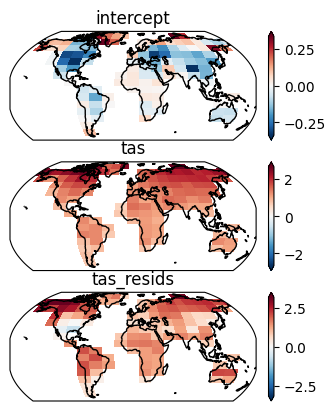
Local variability#
Next we to fit the parameters for the local AR(1) process with a spatially correlated noise term used to emulate local variability:
\(\eta_{s,\,t} = \gamma_{0,\,s} + \gamma_{1,\,s} \cdot \eta_{s,\,t-1} + \nu_{s,\,t}, \ \nu_{s,\,t} \sim \mathcal{N}(0, \Sigma_{\nu}(r))\)
The first component which contains the AR parameters (\(\gamma_{0,\,s} + \gamma_{1,\,2} \cdot \eta_{s,\,t-1}\)) ensures temporal correlation of the local variability whereas the noise term \(\nu_{s,\,t}\) ensures spatial consistency. The covariance matrix \(\Sigma_{\nu}(r)\) is estimated on the whole grid and represents the spatial correlation of temperatures between the different gridpoints.
Estimate the AR parameters#
First we need to compute the residuals after the linear regression.
resids = local_lin_reg.residuals(predictors, target)
The local AR(1) process is estimated on the individual scenarios, but the covariance is estimated on the pooled residuals - therefore we need to have them in both forms.
resids_pooled = mesmer.datatree.pool_scen_ens(resids)
# fit the AR(1) process
local_ar = mesmer.stats.fit_auto_regression_scen_ens(
    resids,
    ens_dim="member",
    dim="time",
    lags=1,
)

local_ar
<xarray.Dataset> Size: 6kB
Dimensions:    (gridcell: 118, lags: 1)
Coordinates:
    lat        (gridcell) float64 944B -49.5 -40.5 -31.5 ... 76.5 76.5 76.5
    lon        (gridcell) float64 944B 288.0 288.0 18.0 ... 306.0 324.0 342.0
  * lags       (lags) int64 8B 1
Dimensions without coordinates: gridcell
Data variables:
    intercept  (gridcell) float64 944B 0.005616 -0.004654 ... 0.001157 -0.008397
    coeffs     (gridcell, lags) float64 944B 0.04741 -0.02513 ... 0.1311 0.2302
    variance   (gridcell) float64 944B 0.1496 0.1605 0.1024 ... 0.8005 0.7438
nobs (gridcell) float64 944B 111.3 111.3 111.3 ... 111.3 111.3 111.3- gridcell: 118
- lags: 1
- lat(gridcell)float64-49.5 -40.5 -31.5 ... 76.5 76.5
- standard_name :
- latitude
- long_name :
- latitude
- units :
- degrees_north
- axis :
- Y
array([-49.5, -40.5, -31.5, -31.5, -31.5, -31.5, -31.5, -22.5, -22.5, -22.5, -22.5, -22.5, -22.5, -13.5, -13.5, -13.5, -13.5, -13.5, -13.5, -4.5, -4.5, -4.5, -4.5, -4.5, -4.5, 4.5, 4.5, 4.5, 4.5, 4.5, 13.5, 13.5, 13.5, 13.5, 13.5, 13.5, 22.5, 22.5, 22.5, 22.5, 22.5, 22.5, 22.5, 22.5, 22.5, 31.5, 31.5, 31.5, 31.5, 31.5, 31.5, 31.5, 31.5, 31.5, 40.5, 40.5, 40.5, 40.5, 40.5, 40.5, 40.5, 40.5, 40.5, 40.5, 40.5, 40.5, 49.5, 49.5, 49.5, 49.5, 49.5, 49.5, 49.5, 49.5, 49.5, 49.5, 49.5, 49.5, 58.5, 58.5, 58.5, 58.5, 58.5, 58.5, 58.5, 58.5, 58.5, 58.5, 58.5, 58.5, 58.5, 58.5, 58.5, 67.5, 67.5, 67.5, 67.5, 67.5, 67.5, 67.5, 67.5, 67.5, 67.5, 67.5, 67.5, 67.5, 67.5, 67.5, 67.5, 67.5, 67.5, 76.5, 76.5, 76.5, 76.5, 76.5, 76.5, 76.5]) - lon(gridcell)float64288.0 288.0 18.0 ... 324.0 342.0
- standard_name :
- longitude
- long_name :
- longitude
- units :
- degrees_east
- axis :
- X
array([288., 288., 18., 126., 144., 288., 306., 18., 36., 126., 144., 288., 306., 18., 36., 126., 288., 306., 324., 18., 36., 144., 288., 306., 324., 0., 18., 36., 288., 306., 0., 18., 36., 108., 270., 342., 0., 18., 36., 54., 72., 90., 108., 252., 342., 0., 18., 36., 54., 72., 90., 108., 252., 270., 0., 18., 36., 54., 72., 90., 108., 126., 234., 252., 270., 288., 0., 18., 36., 54., 72., 90., 108., 126., 234., 252., 270., 288., 18., 36., 54., 72., 90., 108., 126., 144., 162., 198., 216., 234., 252., 270., 288., 18., 36., 54., 72., 90., 108., 126., 144., 162., 180., 198., 216., 234., 252., 270., 288., 306., 324., 90., 108., 270., 288., 306., 324., 342.]) - lags(lags)int641
array([1])
- intercept(gridcell)float640.005616 -0.004654 ... -0.008397
array([ 0.00561619, -0.00465365, 0.00311368, 0.0004456 , -0.00210623, -0.00174239, -0.00898204, -0.00772085, -0.01410007, -0.0024298 , -0.00088733, -0.00241852, -0.01560429, -0.00508964, -0.00444101, 0.00318045, 0.00323338, -0.01553699, 0.00120528, 0.00255577, 0.00060573, 0.0022453 , -0.00531938, -0.03309943, 0.00306931, 0.00022062, 0.00277298, 0.00469052, -0.01041103, -0.00581373, -0.01135155, -0.00469935, -0.00023163, -0.0017558 , -0.00214057, 0.00695244, -0.00480377, -0.00618954, 0.00188409, 0.00355031, -0.00549028, -0.00876583, -0.0114815 , -0.00026629, -0.00072525, -0.00702186, -0.01335862, -0.0109683 , 0.00401961, -0.01991114, -0.04330351, -0.00141621, 0.00433187, -0.00312031, 0.00236735, -0.0067703 , -0.00818825, 0.00303747, -0.00750182, -0.00671081, -0.00069049, -0.00335834, 0.00957269, 0.00740299, 0.01849639, -0.0013816 , -0.0075541 , -0.0038023 , -0.00591696, 0.00275943, -0.01515822, -0.01241976, -0.01764859, -0.00383067, 0.00954064, -0.0182965 , -0.00542471, -0.00564298, 0.00644342, 0.00234624, -0.00290739, -0.0046779 , -0.01093557, -0.00418937, 0.00323987, 0.04552635, 0.03135576, 0.02389307, 0.00408576, 0.00938518, -0.01561875, 0.01687042, -0.00912226, -0.00403992, 0.00520801, 0.02073816, 0.00789627, 0.00141472, 0.00787575, 0.00729357, 0.00489943, 0.01210101, 0.0199518 , 0.02475097, 0.02564096, 0.02618174, 0.01204074, 0.02990142, 0.00847334, 0.02748529, -0.01997084, 0.06355795, 0.01421549, 0.00028313, 0.02319369, 0.00863718, 0.00115651, -0.00839693]) - coeffs(gridcell, lags)float640.04741 -0.02513 ... 0.1311 0.2302
array([[ 0.04741454], [-0.02513218], [ 0.07985752], [ 0.09228125], [ 0.10752609], [ 0.01834117], [ 0.04980009], [ 0.11791813], [-0.04159915], [ 0.05234217], [ 0.04516985], [ 0.14932623], [ 0.01914352], [ 0.16609014], [ 0.02391113], [ 0.02715478], [ 0.23956484], [ 0.07830771], [ 0.27218729], [ 0.2320959 ], ... [ 0.07786044], [ 0.15437376], [ 0.10880347], [ 0.07987162], [ 0.12523694], [ 0.12927414], [ 0.06864319], [ 0.00592539], [ 0.12807239], [ 0.15503393], [ 0.21313706], [ 0.43393415], [ 0.14144758], [ 0.30796548], [ 0.34052578], [ 0.31292227], [ 0.34356902], [ 0.11964258], [ 0.13113206], [ 0.2301981 ]]) - variance(gridcell)float640.1496 0.1605 ... 0.8005 0.7438
array([0.14958378, 0.16053182, 0.10244127, 0.1345089 , 0.16977383, 0.08626104, 0.23259787, 0.12311681, 0.06484364, 0.30326924, 0.25393224, 0.10650618, 0.232044 , 0.08972506, 0.06115187, 0.06014982, 0.03992123, 0.08599044, 0.0472857 , 0.03160961, 0.02642992, 0.00944165, 0.02938985, 0.07963419, 0.02302353, 0.01879353, 0.0184855 , 0.09300582, 0.06516506, 0.0264742 , 0.11329394, 0.14331852, 0.11087922, 0.04470327, 0.03358446, 0.14249218, 0.14519979, 0.20167193, 0.109781 , 0.13301792, 0.11077271, 0.11003088, 0.17459186, 0.08587831, 0.10475902, 0.19330211, 0.09323245, 0.19428241, 0.38715893, 0.33160309, 0.69702913, 0.29767548, 0.30553576, 0.31812631, 0.21788498, 0.21972482, 0.30022013, 0.34316636, 0.41927822, 0.29462829, 0.39981056, 0.36681466, 0.21671681, 0.33166347, 0.54457315, 0.36091054, 0.29806972, 0.52034184, 0.88298016, 0.91051625, 0.867867 , 0.73425058, 0.76528411, 0.43839197, 0.49392842, 0.87239189, 0.4998008 , 0.45695236, 0.76628351, 1.1747903 , 1.07187208, 1.10707714, 1.12503315, 0.85900201, 0.5619434 , 0.55082346, 0.51801134, 1.12262769, 0.51589986, 1.06693212, 0.914054 , 0.64673559, 0.81343419, 0.62789266, 0.78814709, 1.29222848, 1.48562155, 1.08029413, 0.87590402, 0.56610715, 0.65160435, 1.01482385, 1.00910969, 1.06306573, 1.02185256, 1.06500476, 0.8683779 , 0.9073161 , 1.24601168, 1.82460788, 0.49907236, 1.43218476, 1.21875342, 0.9647934 , 1.11540731, 0.94758559, 0.80053245, 0.74382184]) - nobs(gridcell)float64111.3 111.3 111.3 ... 111.3 111.3
array([111.33333333, 111.33333333, 111.33333333, 111.33333333,
       111.33333333, 111.33333333, 111.33333333, 111.33333333,
       111.33333333, 111.33333333, 111.33333333, 111.33333333,
       111.33333333, 111.33333333, 111.33333333, 111.33333333,
       111.33333333, 111.33333333, 111.33333333, 111.33333333,
       111.33333333, 111.33333333, 111.33333333, 111.33333333,
       111.33333333, 111.33333333, 111.33333333, 111.33333333,
       111.33333333, 111.33333333, 111.33333333, 111.33333333,
       111.33333333, 111.33333333, 111.33333333, 111.33333333,
       111.33333333, 111.33333333, 111.33333333, 111.33333333,
       111.33333333, 111.33333333, 111.33333333, 111.33333333,
       111.33333333, 111.33333333, 111.33333333, 111.33333333,
       111.33333333, 111.33333333, 111.33333333, 111.33333333,
       111.33333333, 111.33333333, 111.33333333, 111.33333333,
       111.33333333, 111.33333333, 111.33333333, 111.33333333,
       111.33333333, 111.33333333, 111.33333333, 111.33333333,
       111.33333333, 111.33333333, 111.33333333, 111.33333333,
       111.33333333, 111.33333333, 111.33333333, 111.33333333,
       111.33333333, 111.33333333, 111.33333333, 111.33333333,
       111.33333333, 111.33333333, 111.33333333, 111.33333333,
       111.33333333, 111.33333333, 111.33333333, 111.33333333,
       111.33333333, 111.33333333, 111.33333333, 111.33333333,
       111.33333333, 111.33333333, 111.33333333, 111.33333333,
       111.33333333, 111.33333333, 111.33333333, 111.33333333,
       111.33333333, 111.33333333, 111.33333333, 111.33333333,
       111.33333333, 111.33333333, 111.33333333, 111.33333333,
       111.33333333, 111.33333333, 111.33333333, 111.33333333,
       111.33333333, 111.33333333, 111.33333333, 111.33333333,
       111.33333333, 111.33333333, 111.33333333, 111.33333333,
       111.33333333, 111.33333333])
- lagsPandasIndex
PandasIndex(Index([1], dtype='int64', name='lags'))
Estimate covariance matrix#
For the covariance matrix of the white noise we first estimate the empirical covariance matrix of the gridcell’s values and then localize it using the Gaspari-Cohn function. This function goes to 0 for for larger distances and becomes exactly 0 for distances twice the so called localisation radius. This is also called regularization. It ensures that grid points that are further away from each other do not correlate. Such spurious correlations can arise from rank deficient covariance matrices. In our case because we estimate the covariance on data that has more gridcells than timesteps.
The localisation radius is a parameter that needs to be calibrated and we find the best localisation radius by cross-validation of several radii using the negative loglikelihood.
Prepare the distance matrix - the distance between the gridpoints in km.
grid_stacked = resids["historical"].ds[["lat", "lon"]]
geodist = mesmer.geospatial.geodist_exact(grid_stacked.lon, grid_stacked.lat)

# plot
f, ax = plt.subplots()
geodist.plot(ax=ax, cmap="Blues")

ax.set_aspect("equal")
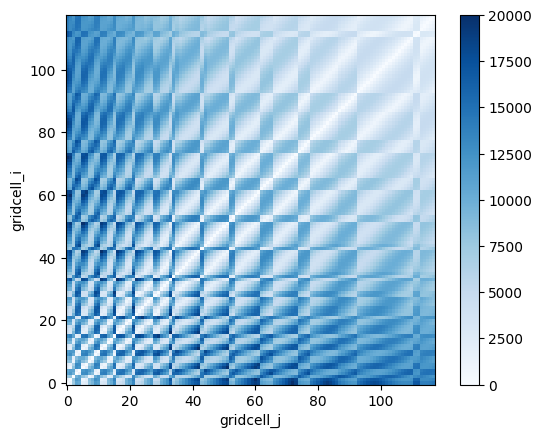
prepare the localizer(s) to regularize the covariance matrix
phi_gc_localizer = mesmer.stats.gaspari_cohn_correlation_matrices(
    geodist, range(5_000, 15_001, 500)
)

# plot one
f, ax = plt.subplots()
phi_gc_localizer[5000].plot(ax=ax, cmap="Blues")

ax.set_aspect("equal")
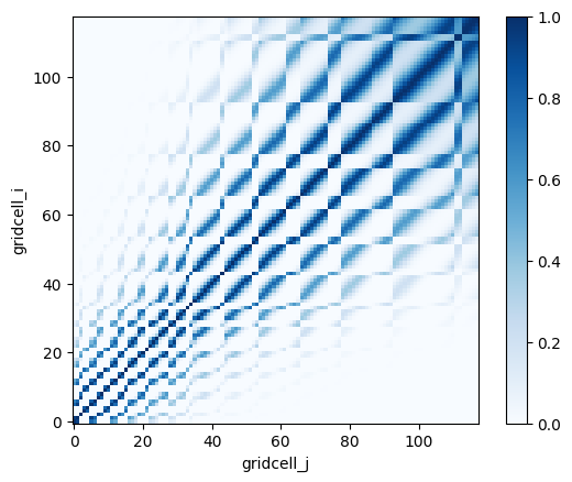
Compute the weights
# reusing weights from local trend regression
find the best localization radius and localize the empirical covariance matrix
dim = "sample"
k_folds = 15

localized_ecov = mesmer.stats.find_localized_empirical_covariance(
    resids_pooled.residuals,
    weights_pooled.weights,
    phi_gc_localizer,
    dim,
    k_folds=k_folds,
)

localized_ecov
<xarray.Dataset> Size: 223kB
Dimensions:               (gridcell_i: 118, gridcell_j: 118)
Dimensions without coordinates: gridcell_i, gridcell_j
Data variables:
    localization_radius   int64 8B 12500
    covariance            (gridcell_i, gridcell_j) float64 111kB 0.1585 ... 0...
localized_covariance (gridcell_i, gridcell_j) float64 111kB 0.1585 ... 0...- gridcell_i: 118
- gridcell_j: 118
- localization_radius()int6412500
array(12500)
- covariance(gridcell_i, gridcell_j)float640.1585 0.112 ... 0.1602 0.8493
array([[ 1.58512649e-01, 1.11954928e-01, 1.25712271e-02, ..., 2.42374317e-02, 1.34521129e-02, -1.60513480e-02], [ 1.11954928e-01, 1.62869525e-01, 5.50508230e-03, ..., 5.00106398e-03, 4.31114508e-03, -9.19310862e-04], [ 1.25712271e-02, 5.50508230e-03, 1.05823006e-01, ..., 4.12977354e-03, 5.19339310e-03, -4.02591382e-02], ..., [ 2.42374317e-02, 5.00106398e-03, 4.12977354e-03, ..., 9.81592283e-01, 8.10685547e-01, 1.27054591e-01], [ 1.34521129e-02, 4.31114508e-03, 5.19339310e-03, ..., 8.10685547e-01, 8.61498003e-01, 1.60220960e-01], [-1.60513480e-02, -9.19310862e-04, -4.02591382e-02, ..., 1.27054591e-01, 1.60220960e-01, 8.49310934e-01]], shape=(118, 118)) - localized_covariance(gridcell_i, gridcell_j)float640.1585 0.1108 ... 0.1599 0.8493
array([[ 1.58512649e-01,  1.10798346e-01,  7.37986590e-03, ...,
         3.19833215e-03,  1.67739464e-03, -1.82366883e-03],
       [ 1.10798346e-01,  1.62869525e-01,  3.04688128e-03, ...,
         8.94969937e-04,  7.31230697e-04, -1.42855566e-04],
       [ 7.37986590e-03,  3.04688128e-03,  1.05823006e-01, ...,
         7.62437931e-04,  1.06958259e-03, -8.99597287e-03],
       ...,
       [ 3.19833215e-03,  8.94969937e-04,  7.62437931e-04, ...,
         9.81592283e-01,  8.08823458e-01,  1.25931536e-01],
       [ 1.67739464e-03,  7.31230697e-04,  1.06958259e-03, ...,
         8.08823458e-01,  8.61498003e-01,  1.59852943e-01],
       [-1.82366883e-03, -1.42855566e-04, -8.99597287e-03, ...,
         1.25931536e-01,  1.59852943e-01,  8.49310934e-01]],
      shape=(118, 118))
f, axs = plt.subplots(1, 2, sharey=True, constrained_layout=True)

opt = dict(vmin=0, vmax=1.5, cmap="Blues", add_colorbar=False)

ax = axs[0]
localized_ecov.covariance.plot(ax=ax, **opt)
ax.set_aspect("equal")
ax.set_title("Empirical covariance")

ax = axs[1]
localized_ecov.localized_covariance.plot(ax=ax, **opt)
ax.set_aspect("equal")
ax.set_title("Localized empirical covariance")
ax.set_ylabel("")
plt.show()
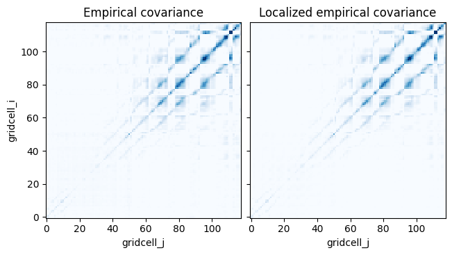
Adjust the regularized covariance matrix
Lastly we need to adjust the localized covariance matrix using the AR(1) parameters since the variance of the time series we observe is bigger than the variance of the driving white noise process. Read more about this in: “Statistical Analysis in Climate Research” by Storch and Zwiers (1999, reprinted 2003).
localized_covariance_adjusted = mesmer.stats.adjust_covariance_ar1(
    localized_ecov.localized_covariance, local_ar.coeffs
)
Saving the parameters#
Finally, we have calibrated all needed parameters and can save them. We can use filefisher to nicely create file names and save the parameters.
# define path relative to this notebook & create folder
param_path = pathlib.Path("./output/calibrated_parameters/")
PARAM_FILEFINDER = filefisher.FileFinder(
    path_pattern=param_path / "{esm}_{scen}",
    file_pattern="params_{module}_{esm}_{scen}.nc",
)

scen_str = "-".join(scenarios)

folder = PARAM_FILEFINDER.create_path_name(esm=model, scen=scen_str)
pathlib.Path(folder).mkdir(exist_ok=True, parents=True)

params = {
    "volcanic": volcanic_params,
    "global-variability": global_ar_params,
    "local-trends": local_lin_reg,
    "local-variability": local_ar,
    "covariance": localized_ecov,
    "grid-orig": grid_orig,
}


save_files = False  # we don't save them here in the example
if save_files:

    for module, param in params.items():

        filename = PARAM_FILEFINDER.create_full_name(
            module=module,
            esm=model,
            scen=scen_str,
        )

        param.to_netcdf(filename)
When you want to use the calibrated parameters for emulation, see the Tutorials for emulating one or multiple scenarios in the Tutorial section next.