Note

This page was generated from an Jupyter notebook that can be accessed from github.

Emulating near surface temperature on land with MESMER

Using calibrated parameters, we can emulate a large ensemble of realisations of near surface temperature with MESMER. To calibrate MESMER, follow the tutorials on calibrating either multiple scenarios in the Tutorial section. Here, we will emulate realisation for two scenarios predicting global mean temperature trajectories at once.

import pathlib

import cartopy.crs as ccrs
import filefisher
import matplotlib.pyplot as plt
import xarray as xr

import mesmer

Load forcing data

One can use any global mean temperature trajectory to draw gridded realisations. For this example we want to create emulations for SSP1-2.6 and SSP5-8.5 to compare the emulations to the actual ESM output. Here we concatenate historical and future simulations to create a continuous timeseries.

model = "IPSL-CM6A-LR"
scenarios = ["ssp126", "ssp585"]

# some configuration parameters
THRESHOLD_LAND = 1 / 3

REFERENCE_PERIOD = slice("1850", "1900")

HIST_PERIOD = slice("1850", "2014")

cmip_path = mesmer.example_data.cmip6_ng_path(relative=True)

CMIP_FILEFINDER = filefisher.FileFinder(
    path_pattern=cmip_path / "{variable}/{time_res}/{resolution}",
    file_pattern="{variable}_{time_res}_{model}_{scenario}_{member}_{resolution}.nc",
)

keys = {"variable": "tas", "model": model, "resolution": "g025", "time_res": "ann"}

fc_scens = CMIP_FILEFINDER.find_files(keys, scenario=scenarios)

members = fc_scens.df.member.unique()

fc_hist = CMIP_FILEFINDER.find_files(keys, scenario="historical", member=members)

def _get_hist(meta, fc_hist):

    meta_hist = meta | {"scenario": "historical"}

    fc = fc_hist.search(**meta_hist)

    if len(fc) == 0:
        raise FileNotFoundError("no hist file found")
    if len(fc) != 1:
        raise ValueError("more than one hist file found")

    fN, meta_hist = fc[0]

    return fN, meta_hist


def load_hist(meta, fc_hist):
    fN, __ = _get_hist(meta, fc_hist)

    time_coder = xr.coders.CFDatetimeCoder(use_cftime=True)
    return xr.open_dataset(fN, decode_times=time_coder)


def load_hist_scen_continuous(fc_hist, fc_scens):
    dt = xr.DataTree()
    for scen in fc_scens.df.scenario.unique():
        files = fc_scens.search(scenario=scen)

        members = []

        time_coder = xr.coders.CFDatetimeCoder(use_cftime=True)

        for fN, meta in files.items():

            try:
                hist = load_hist(meta, fc_hist)
            except FileNotFoundError:
                continue

            proj = xr.open_dataset(fN, decode_times=time_coder)

            ds = xr.combine_by_coords(
                [hist, proj],
                combine_attrs="override",
                data_vars="minimal",
                compat="override",
                coords="minimal",
            )

            ds = ds.drop_vars(("height", "time_bnds", "file_qf"), errors="ignore")

            # assign member-ID as coordinate
            ds = ds.assign_coords({"member": meta["member"]})

            members.append(ds)

        # create a Dataset that holds each member along the member dimension
        scen_data = xr.concat(members, dim="member")
        # put the scenario dataset into the DataTree
        dt[scen] = xr.DataTree(scen_data)
    return dt

Pre-process temperature data

# load data
tas = load_hist_scen_continuous(fc_hist, fc_scens)
# calculate anomalies w.r.t. the reference period
ref = tas.sel(time=REFERENCE_PERIOD).mean("time")
tas_anom = tas - ref
# calculate global mean
tas_globmean = mesmer.weighted.global_mean(tas_anom)

# calculate smooth ensemble mean
tas_globmean_ensmean = tas_globmean.mean(dim="member")
tas_globmean_forcing = mesmer.stats.lowess(
    tas_globmean_ensmean,
    dim="time",
    n_steps=30,
    use_coords=False,
)
time = tas_globmean_forcing["ssp126"].time

Load the parameters

We load the parameters that were calibrated on historical, SSP1-2.6 and SSP5-8.5 data. But one can also use parameters that were calibrated on only one scenario. For more details on the benefits of calibrating on multiple scenarios, please refer to Beusch et al. (2022).

# find the parameters - use same relative path as above
data_path = pathlib.Path("./output/calibrated_parameters/")

PARAM_FILEFINDER = filefisher.FileFinder(
    path_pattern=data_path / "{esm}_{scen}",
    file_pattern="params_{module}_{esm}_{scen}.nc",
)

param_files = PARAM_FILEFINDER.find_files(esm=model)
param_files.df

	esm	scen	module
path
output/calibrated_parameters/IPSL-CM6A-LR_ssp126-ssp585/params_covariance_IPSL-CM6A-LR_ssp126-ssp585.nc	IPSL-CM6A-LR	ssp126-ssp585	covariance
output/calibrated_parameters/IPSL-CM6A-LR_ssp126-ssp585/params_global-variability_IPSL-CM6A-LR_ssp126-ssp585.nc	IPSL-CM6A-LR	ssp126-ssp585	global-variability
output/calibrated_parameters/IPSL-CM6A-LR_ssp126-ssp585/params_grid-orig_IPSL-CM6A-LR_ssp126-ssp585.nc	IPSL-CM6A-LR	ssp126-ssp585	grid-orig
output/calibrated_parameters/IPSL-CM6A-LR_ssp126-ssp585/params_local-trends_IPSL-CM6A-LR_ssp126-ssp585.nc	IPSL-CM6A-LR	ssp126-ssp585	local-trends
output/calibrated_parameters/IPSL-CM6A-LR_ssp126-ssp585/params_local-variability_IPSL-CM6A-LR_ssp126-ssp585.nc	IPSL-CM6A-LR	ssp126-ssp585	local-variability
output/calibrated_parameters/IPSL-CM6A-LR_ssp126-ssp585/params_volcanic_IPSL-CM6A-LR_ssp126-ssp585.nc	IPSL-CM6A-LR	ssp126-ssp585	volcanic

Where scen denotes the scenarios on which the parameters where fitted on. In this example we create emulations using the global mean temperature forcing from the same scenarios, however, this does not necessarily need to be the case!

all_modules = [
    "volcanic",
    "global-variability",
    "local-trends",
    "local-variability",
    "covariance",
]

params = xr.DataTree()

for module in all_modules:
    params[module] = xr.DataTree(
        xr.open_dataset(param_files.search(module=module).paths.pop()), name=module
    )

Define seeds for global and local variability

If we want reproducible results we need to set a seed for the random samples of global and local variability. Here, we set the seed to a chosen number, but for automated generation of seeds i.e. for several ESM we recommend using the secrets from the standard library. Then you would generate a seed using:

import secrets

secrets.randbits(64)

For reproducibility the same seeds need to be used every time, so you would copy the generated seeds to keep them unique but constant.

seed_global_variability = xr.DataTree.from_dict(
    {
        "ssp126": xr.Dataset(data_vars={"seed": 981}),
        "ssp585": xr.Dataset(data_vars={"seed": 314}),
    }
)
seed_local_variability = xr.DataTree.from_dict(
    {
        "ssp126": xr.Dataset(data_vars={"seed": 272}),
        "ssp585": xr.Dataset(data_vars={"seed": 42}),
    }
)

Make emulations

# some settings
n_realisations = 10

buffer_global_variability = 50
buffer_local_variability = 20

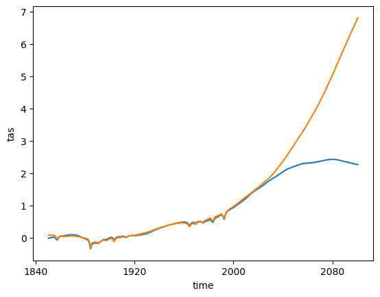
1. Adding the volcanic influence to the smooth global mean forcing

This is optional, depending on if the used temperature forcing dataset contains a volcanic signal or not and if you want to reproduce it in the historical period. This is necessary when we want to evaluate the performance of our emulator on ESM or observation data but might not be necessary for more abstract research questions.

tas_globmean_forcing_volc = mesmer.volc.superimpose_volcanic_influence(
    tas_globmean_forcing,
    params["volcanic"].ds,
    hist_period=HIST_PERIOD,
)

tas_globmean_forcing_volc["ssp126"].to_dataset().tas.plot()
tas_globmean_forcing_volc["ssp585"].to_dataset().tas.plot()

[<matplotlib.lines.Line2D at 0x7ebe7d93ba70>]

2. Compute global variabilty

Draw samples from a AR process with the calibrated parameters.

global_variability = mesmer.stats.draw_auto_regression_uncorrelated(
    params["global-variability"].ds,
    realisation=n_realisations,
    time=time,
    seed=seed_global_variability,
    buffer=buffer_global_variability,
)
global_variability = mesmer.datatree.map_over_datasets(
    lambda ds: ds.rename({"samples": "tas_resids"}), global_variability
)

3. Compute local forced response

Apply linear regression using the global mean forcing and the global variability as predictors. Optionally, you can also add other variables to the predictors like ocean heat content or squared global mean temperature.

predictors = mesmer.datatree.merge([tas_globmean_forcing_volc, global_variability])

lr_params = params["local-trends"].ds
lr = mesmer.stats.LinearRegression.from_params(lr_params)

# uses ``exclude`` to split the linear response
local_forced_response = lr.predict(predictors, exclude={"tas_resids"})

# local variability part driven by global variabilty - only from `tas_resids`
local_variability_from_global_var = lr.predict(predictors, only={"tas_resids"})

4. Compute local variability

We compute the local variability by applying an AR(1) process to ensure consistency in time and adding spatially correlated innovations at each time step to get spatially coherent random samples at each gridpoint.

local_variability = mesmer.stats.draw_auto_regression_correlated(
    params["local-variability"].ds,
    params["covariance"].localized_covariance,
    time=time,
    realisation=n_realisations,
    seed=seed_local_variability,
    buffer=buffer_local_variability,
)
local_variability = mesmer.datatree.map_over_datasets(
    lambda ds: ds.rename({"samples": "prediction"}), local_variability
)

5. Add everything together

local_variability_total = local_variability_from_global_var + local_variability
emulations = local_forced_response + local_variability_total

emulations = mesmer.datatree.map_over_datasets(
    lambda ds: ds.rename({"prediction": "tas"}),
    emulations,
)

Saving emulations

We recommend saving the emulations together with the seeds used for emulating.

for scen in emulations:
    local_seed = seed_local_variability[scen].seed.rename("seed_local_variability")
    global_seed = seed_global_variability[scen].seed.rename("seed_global_variability")
    emulations[scen] = xr.DataTree(
        xr.merge([emulations[scen].ds, local_seed, global_seed])
    )

path = "./output/emulations/"
# uncomment to save emulations
# emulations.to_netcdf(path + f"tas_emulations_{model}_ssp126-ssp585.nc")

Some example plots

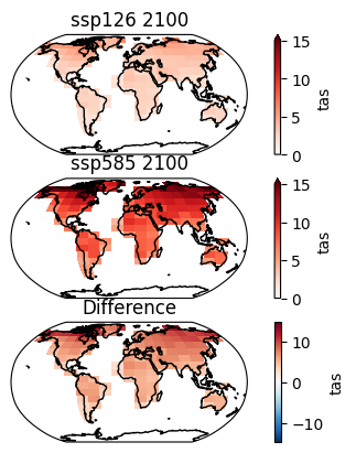
# maps of the means over all realisations for the two scenarios and their difference in 2100
grid_orig = tas_anom["ssp126"].ds[["lat", "lon"]]
spatial_emu_126 = mesmer.grid.unstack_lat_lon_and_align(
    emulations["ssp126"].tas, grid_orig
)
spatial_emu_585 = mesmer.grid.unstack_lat_lon_and_align(
    emulations["ssp585"].tas, grid_orig
)

f, axs = plt.subplots(3, 1, subplot_kw={"projection": ccrs.Robinson()})

opt = dict(cmap="Reds", transform=ccrs.PlateCarree(), vmin=0, vmax=15, extend="max")
spatial_emu_126.mean("realisation").sel(time="2100").plot(ax=axs[0], **opt)
spatial_emu_585.mean("realisation").sel(time="2100").plot(ax=axs[1], **opt)

diff = spatial_emu_585 - spatial_emu_126
diff.mean("realisation").sel(time="2100").plot(
    ax=axs[2], cmap="RdBu_r", transform=ccrs.PlateCarree(), center=0
)

axs[0].set_title("ssp126 2100")
axs[1].set_title("ssp585 2100")
axs[2].set_title("Difference")

for ax in axs:
    ax.coastlines()
    ax.set_global()

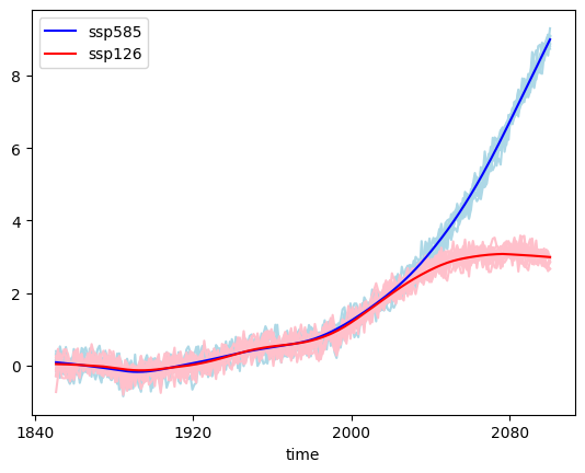
# plot global land means
globmean_126 = mesmer.weighted.global_mean(spatial_emu_126)
globmean_585 = mesmer.weighted.global_mean(spatial_emu_585)

globmean_126_smoothed = mesmer.stats.lowess(
    globmean_126.mean("realisation"), dim="time", n_steps=50, use_coords=False
)
globmean_585_smoothed = mesmer.stats.lowess(
    globmean_585.mean("realisation"), dim="time", n_steps=50, use_coords=False
)

f, ax = plt.subplots()
globmean_585.plot.line(x="time", ax=ax, add_legend=False, color="lightblue")
globmean_126.plot.line(x="time", ax=ax, add_legend=False, color="pink")

globmean_585_smoothed.plot.line(x="time", ax=ax, color="blue", label="ssp585")
globmean_126_smoothed.plot.line(x="time", ax=ax, color="red", label="ssp126")

plt.legend()
plt.show()

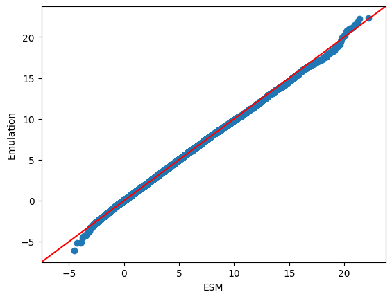
# qq plot between ESM and emulation
esm_ssp585 = tas_anom["ssp585"].ds


def mask(ds, threshold_land):
    ds = mesmer.mask.mask_ocean_fraction(ds, threshold_land)
    ds = mesmer.mask.mask_antarctica(ds)
    return ds


esm_ssp585 = mask(esm_ssp585, THRESHOLD_LAND)

esm_ssp585 = esm_ssp585.tas.stack(sample=("time", "lat", "lon", "member"))
emu_ssp585 = spatial_emu_585.stack(sample=("time", "lat", "lon", "realisation"))

import statsmodels.api as sm

sm.qqplot_2samples(esm_ssp585, emu_ssp585, line="45")
plt.xlabel("ESM")
plt.ylabel("Emulation")
plt.show()