Note
This page was generated from an Jupyter notebook that can be accessed from github.
MESMER-M: calibrate multiple scenarios#
Training monthly local temperature from yearly local temperature for multiple scenarios and ensemble members. We use an example data set on a coarse grid. This roughly follows the approach outlined in Nath et al. (2022).
MESMER-M trains the local monthly temperature using the local annual temperature (i.e. the temperature from the same grid point) as forcing. This is different from MESMER which uses global mean values as predictors for where local annual mean temperatures. Training MESMER-M consists of 4 steps:
harmonic model: fit the seasonal cycle with a harmonic model
power transformer: make the resulting residuals more normal by using a Yeo-Johnson transformation
cyclo-stationary AR(1) process: the monthly residuals are assumed to follow a cyclo-stationary AR(1) process, where one months value depends on the previous one
local variability: estimate parameters needed to generate local variability
This example can be extended to more scenarios, ensemble members and higher resolution data. See also the MESMER-M calibration and emulation tests in tests/integration/.
import pathlib

import filefisher
import matplotlib.pyplot as plt
import pandas as pd
import scipy as sp
import xarray as xr

import mesmer
Configuration#
# target model
model = "IPSL-CM6A-LR"

# scenarios used for training
scenarios = ["ssp126", "ssp585"]

# gridcells considered as land
THRESHOLD_LAND = 1 / 3

# reference period
REFERENCE_PERIOD = slice("1850", "1900")

# localisation radius for covariance matrix
LOCALISATION_RADII = list(range(7_500, 12_501, 500))

# path of the example data
# NOTE: this downloads the tutorial data and caches it locally if needed
cmip6_data_path = mesmer.example_data.cmip6_ng_path(relative=True)

# mesmer-m downscales annual temperature to
# monthly resolution

# variable, shared for input and output
variable = "tas"

# spatial resolution, shared for input and output
spatial_resolution = "g025"

# targeted temporal resolution
temporal_resolution_target = "mon"

# temporal resolution of the forcing data
temporal_resolution_forcing = "ann"
Load Data#
We search monthly and annual mean temperatures using the library filefisher
CMIP_FILEFINDER = filefisher.FileFinder(
    path_pattern=cmip6_data_path / "{variable}/{time_res}/{resolution}",
    file_pattern="{variable}_{time_res}_{model}_{scenario}_{member}_{resolution}.nc",
)
We search for the initial (annual) data for ssp126 and ssp585 as well as the corresponding historical data:
fc_scens_y = CMIP_FILEFINDER.find_files(
    variable=variable,
    scenario=scenarios,
    model=model,
    resolution=spatial_resolution,
    time_res=temporal_resolution_forcing,
)

# get the historical members that are also in the future scenarios, but only once
unique_scen_members_y = fc_scens_y.df.member.unique()

fc_hist_y = CMIP_FILEFINDER.find_files(
    variable=variable,
    scenario="historical",
    model=model,
    resolution=spatial_resolution,
    time_res=temporal_resolution_forcing,
    member=unique_scen_members_y,
)

fc_all_y = fc_hist_y.concat(fc_scens_y)
fc_all_y.df
| variable | time_res | resolution | model | scenario | member | |
|---|---|---|---|---|---|---|
| path | ||||||
| ../data/cmip6-ng/tas/ann/g025/tas_ann_IPSL-CM6A-LR_historical_r1i1p1f1_g025.nc | tas | ann | g025 | IPSL-CM6A-LR | historical | r1i1p1f1 |
| ../data/cmip6-ng/tas/ann/g025/tas_ann_IPSL-CM6A-LR_historical_r2i1p1f1_g025.nc | tas | ann | g025 | IPSL-CM6A-LR | historical | r2i1p1f1 |
| ../data/cmip6-ng/tas/ann/g025/tas_ann_IPSL-CM6A-LR_ssp126_r1i1p1f1_g025.nc | tas | ann | g025 | IPSL-CM6A-LR | ssp126 | r1i1p1f1 |
| ../data/cmip6-ng/tas/ann/g025/tas_ann_IPSL-CM6A-LR_ssp585_r1i1p1f1_g025.nc | tas | ann | g025 | IPSL-CM6A-LR | ssp585 | r1i1p1f1 |
| ../data/cmip6-ng/tas/ann/g025/tas_ann_IPSL-CM6A-LR_ssp585_r2i1p1f1_g025.nc | tas | ann | g025 | IPSL-CM6A-LR | ssp585 | r2i1p1f1 |
Similarly, we search for the target (monthly) data for ssp126 and ssp585 as well as the corresponding historical data:
fc_scens_m = CMIP_FILEFINDER.find_files(
    variable=variable,
    scenario=scenarios,
    model=model,
    resolution=spatial_resolution,
    time_res=temporal_resolution_target,
)

# get the historical members that are also in the future scenarios, but only once
unique_scen_members_m = fc_scens_y.df.member.unique()

fc_hist_m = CMIP_FILEFINDER.find_files(
    variable="tas",
    scenario="historical",
    model=model,
    resolution="g025",
    time_res="mon",
    member=unique_scen_members_m,
)

fc_all_m = fc_hist_m.concat(fc_scens_m)
fc_all_m.df
| variable | time_res | resolution | model | scenario | member | |
|---|---|---|---|---|---|---|
| path | ||||||
| ../data/cmip6-ng/tas/mon/g025/tas_mon_IPSL-CM6A-LR_historical_r1i1p1f1_g025.nc | tas | mon | g025 | IPSL-CM6A-LR | historical | r1i1p1f1 |
| ../data/cmip6-ng/tas/mon/g025/tas_mon_IPSL-CM6A-LR_historical_r2i1p1f1_g025.nc | tas | mon | g025 | IPSL-CM6A-LR | historical | r2i1p1f1 |
| ../data/cmip6-ng/tas/mon/g025/tas_mon_IPSL-CM6A-LR_ssp126_r1i1p1f1_g025.nc | tas | mon | g025 | IPSL-CM6A-LR | ssp126 | r1i1p1f1 |
| ../data/cmip6-ng/tas/mon/g025/tas_mon_IPSL-CM6A-LR_ssp585_r1i1p1f1_g025.nc | tas | mon | g025 | IPSL-CM6A-LR | ssp585 | r1i1p1f1 |
| ../data/cmip6-ng/tas/mon/g025/tas_mon_IPSL-CM6A-LR_ssp585_r2i1p1f1_g025.nc | tas | mon | g025 | IPSL-CM6A-LR | ssp585 | r2i1p1f1 |
This found 1 ensemble member for SSP1-2.6 and two for SSP5-8.5 and the corresponding ones in the historical scenario.
Now we load all the files we found into a DataTree, a data structure provided by xarray. It is a container to hold xarray Dataset objects that are not alignable. This is useful for us since we have historical and future data, which have different time coordinates. Moreover, the scenarios may also have different numbers of members (as e.g., SSP1-2.6, which only has one). Thus, we store the data of each scenario in a Dataset with all its ensemble members along a member dimension. Then we store all the scenario datasets in one DataTree node. The DataTree allows us to perform computations on each of the scenarios separately.
We define a helper function to load the data from the cmip6_ng example data repository:
def load_data(filecontainer):

    out = xr.DataTree()

    scenarios = filecontainer.df.scenario.unique().tolist()

    # load data for each scenario
    for scen in scenarios:
        files = filecontainer.search(scenario=scen)

        # load all members for a scenario
        members = []
        for fN, meta in files.items():
            time_coder = xr.coders.CFDatetimeCoder(use_cftime=True)
            ds = xr.open_dataset(fN, decode_times=time_coder)
            # drop unnecessary variables
            ds = ds.drop_vars(["height", "time_bnds", "file_qf"], errors="ignore")
            # assign member-ID as coordinate
            ds = ds.assign_coords({"member": meta["member"]})
            members.append(ds)

        # create a Dataset that holds each member along the member dimension
        scen_data = xr.concat(members, dim="member")
        # put the scenario dataset into the DataTree
        out[scen] = xr.DataTree(scen_data)

    return out
Load annual (yearly - y) and monthly (m) data:
tas_y_orig = load_data(fc_all_y)
tas_m_orig = load_data(fc_all_m)
This results in two DataTree objects, with 3 nodes, one for each scenario (click on Groups to see the individual Datasets for the three scenarios):
tas_y_orig
<xarray.DataTree>
Group: /
├── Group: /historical
│       Dimensions:  (member: 2, time: 165, lat: 20, lon: 20)
│       Coordinates:
│         * member   (member) <U8 64B 'r1i1p1f1' 'r2i1p1f1'
│         * time     (time) object 1kB 1850-07-01 06:00:00 ... 2014-07-01 06:00:00
│         * lat      (lat) float64 160B -85.5 -76.5 -67.5 -58.5 ... 58.5 67.5 76.5 85.5
│         * lon      (lon) float64 160B 0.0 18.0 36.0 54.0 ... 288.0 306.0 324.0 342.0
│       Data variables:
│           tas      (member, time, lat, lon) float64 1MB 226.3 225.0 ... 258.4 259.6
│       Attributes: (12/56)
│           CDI:                       Climate Data Interface version 1.9.9 (https://...
│           source:                    IPSL-CM6A-LR (2017):  atmos: LMDZ (NPv6, N96; ...
│           institution:               Institut Pierre Simon Laplace, Paris 75252, Fr...
│           Conventions:               CF-1.7 CMIP-6.2
│           history:                   Thu Mar 18 19:05:09 2021: cdo remapbil,r20x20 ...
│           creation_date:             2018-07-11T07:36:34Z
│           ...                        ...
│           realization_index:         1
│           NCO:                       "4.6.0"
│           cmip6-ng:                  \ncontact = cmip6-archive@env.ethz.ch\ndescrip...
│           original_file_names:       /net/atmos/data/cmip6/historical/Amon/tas/IPSL...
│           original_file_hash_codes:  7264c228560257b32d44dcc611d92976da7214af7e8795...
│           CDO:                       Climate Data Operators version 1.9.9 (https://...
├── Group: /ssp126
│       Dimensions:  (member: 1, time: 86, lat: 20, lon: 20)
│       Coordinates:
│         * member   (member) <U8 32B 'r1i1p1f1'
│         * time     (time) object 688B 2015-07-01 06:00:00 ... 2100-07-01 06:00:00
│         * lat      (lat) float64 160B -85.5 -76.5 -67.5 -58.5 ... 58.5 67.5 76.5 85.5
│         * lon      (lon) float64 160B 0.0 18.0 36.0 54.0 ... 288.0 306.0 324.0 342.0
│       Data variables:
│           tas      (member, time, lat, lon) float64 275kB 227.7 226.1 ... 263.4 264.9
│       Attributes: (12/56)
│           CDI:                       Climate Data Interface version 1.9.9 (https://...
│           source:                    IPSL-CM6A-LR (2017):  atmos: LMDZ (NPv6, N96; ...
│           institution:               Institut Pierre Simon Laplace, Paris 75252, Fr...
│           Conventions:               CF-1.7 CMIP-6.2
│           history:                   Thu Mar 18 19:05:09 2021: cdo remapbil,r20x20 ...
│           name:                      /ccc/work/cont003/gencmip6/oboucher/IGCM_OUT/I...
│           ...                        ...
│           dr2xml_md5sum:             c2dce418e78ca835be1e2ff817c2c403
│           model_version:             6.1.8
│           cmip6-ng:                  \ncontact = cmip6-archive@env.ethz.ch\ndescrip...
│           original_file_names:       /net/atmos/data/cmip6/ssp126/Amon/tas/IPSL-CM6...
│           original_file_hash_codes:  8cfb5fd339c050bc81d2e2eeb7263ceec89c295d15631b...
│           CDO:                       Climate Data Operators version 1.9.9 (https://...
└── Group: /ssp585
        Dimensions:  (member: 2, time: 86, lat: 20, lon: 20)
        Coordinates:
          * member   (member) <U8 64B 'r1i1p1f1' 'r2i1p1f1'
          * time     (time) object 688B 2015-07-01 06:00:00 ... 2100-07-01 06:00:00
          * lat      (lat) float64 160B -85.5 -76.5 -67.5 -58.5 ... 58.5 67.5 76.5 85.5
          * lon      (lon) float64 160B 0.0 18.0 36.0 54.0 ... 288.0 306.0 324.0 342.0
        Data variables:
            tas      (member, time, lat, lon) float64 550kB 226.4 225.0 ... 275.5 277.2
        Attributes: (12/56)
            CDI:                       Climate Data Interface version 2.1.0 (https://...
            source:                    IPSL-CM6A-LR (2017):  atmos: LMDZ (NPv6, N96; ...
            institution:               Institut Pierre Simon Laplace, Paris 75252, Fr...
            Conventions:               CF-1.7 CMIP-6.2
            history:                   Wed Oct 26 15:35:08 2022: cdo remapbil,r20x20 ...
            name:                      /ccc/work/cont003/gencmip6/oboucher/IGCM_OUT/I...
            ...                        ...
            dr2xml_md5sum:             c2dce418e78ca835be1e2ff817c2c403
            model_version:             6.1.8
            cmip6-ng:                  \ncontact = cmip6-archive@env.ethz.ch\ndescrip...
            original_file_names:       /net/atmos/data/cmip6/ssp585/Amon/tas/IPSL-CM6...
            original_file_hash_codes:  a2117793ca25ad66f75a37be51fd2e6165c2ba2684b7d4...
CDO: Climate Data Operators version 2.1.0 (https://...Preprocessing#
We will need some configuration parameters in the following:
THRESHOLD_LAND: threshold above which land fraction to consider a grid point as a land grid point.REFERENCE_PERIOD: we will work not with absolute temperature values but with temperature anomalies w.r.t. a reference period
Calculate anomalies#
tas_anoms_y = mesmer.anomaly.calc_anomaly(tas_y_orig, reference_period=REFERENCE_PERIOD)
tas_anoms_m = mesmer.anomaly.calc_anomaly(tas_m_orig, reference_period=REFERENCE_PERIOD)
Extract land gridcells & stack#
We only use land grid points and exclude Antarctica. The 3D data with dimensions ('time', 'lat', 'lon') is stacked to 2D data with dimensions ('time', 'gridcell'):
Before stacking, we extract the original grid. We need to save this together with the parameters to later be able to reconstruct the original grid from the gridpoints.
# extract original grid
grid_orig = tas_anoms_y["historical"].ds[["lat", "lon"]]
def mask_and_stack(ds, threshold_land):
    ds = mesmer.mask.mask_ocean_fraction(ds, threshold_land)
    ds = mesmer.mask.mask_antarctica(ds)
    ds = mesmer.grid.stack_lat_lon(ds)
    return ds
tas_y = mask_and_stack(tas_anoms_y, threshold_land=THRESHOLD_LAND)
tas_m = mask_and_stack(tas_anoms_m, threshold_land=THRESHOLD_LAND)

tas_y
<xarray.DataTree>
Group: /
├── Group: /historical
│       Dimensions:  (member: 2, time: 165, gridcell: 118)
│       Coordinates:
│         * member   (member) <U8 64B 'r1i1p1f1' 'r2i1p1f1'
│         * time     (time) object 1kB 1850-07-01 06:00:00 ... 2014-07-01 06:00:00
│           lat      (gridcell) float64 944B -49.5 -40.5 -31.5 -31.5 ... 76.5 76.5 76.5
│           lon      (gridcell) float64 944B 288.0 288.0 18.0 ... 306.0 324.0 342.0
│       Dimensions without coordinates: gridcell
│       Data variables:
│           tas      (member, time, gridcell) float64 312kB -0.1548 -0.1209 ... 3.151
│       Attributes: (12/56)
│           CDI:                       Climate Data Interface version 1.9.9 (https://...
│           source:                    IPSL-CM6A-LR (2017):  atmos: LMDZ (NPv6, N96; ...
│           institution:               Institut Pierre Simon Laplace, Paris 75252, Fr...
│           Conventions:               CF-1.7 CMIP-6.2
│           history:                   Thu Mar 18 19:05:09 2021: cdo remapbil,r20x20 ...
│           creation_date:             2018-07-11T07:36:34Z
│           ...                        ...
│           realization_index:         1
│           NCO:                       "4.6.0"
│           cmip6-ng:                  \ncontact = cmip6-archive@env.ethz.ch\ndescrip...
│           original_file_names:       /net/atmos/data/cmip6/historical/Amon/tas/IPSL...
│           original_file_hash_codes:  7264c228560257b32d44dcc611d92976da7214af7e8795...
│           CDO:                       Climate Data Operators version 1.9.9 (https://...
├── Group: /ssp126
│       Dimensions:  (member: 1, time: 86, gridcell: 118)
│       Coordinates:
│         * member   (member) <U8 32B 'r1i1p1f1'
│         * time     (time) object 688B 2015-07-01 06:00:00 ... 2100-07-01 06:00:00
│           lat      (gridcell) float64 944B -49.5 -40.5 -31.5 -31.5 ... 76.5 76.5 76.5
│           lon      (gridcell) float64 944B 288.0 288.0 18.0 ... 306.0 324.0 342.0
│       Dimensions without coordinates: gridcell
│       Data variables:
│           tas      (member, time, gridcell) float64 81kB 0.519 0.5718 ... 4.245 5.811
│       Attributes: (12/37)
│           CDI:                   Climate Data Interface version 1.9.9 (https://mpim...
│           source:                IPSL-CM6A-LR (2017):  atmos: LMDZ (NPv6, N96; 144 ...
│           institution:           Institut Pierre Simon Laplace, Paris 75252, France
│           Conventions:           CF-1.7 CMIP-6.2
│           contact:               ipsl-cmip6@listes.ipsl.fr
│           external_variables:    areacella
│           ...                    ...
│           variable_id:           tas
│           variant_info:          Each member starts from the corresponding member o...
│           variant_label:         r1i1p1f1
│           CMIP6_CV_version:      cv=6.2.3.5-2-g63b123e
│           CDO:                   Climate Data Operators version 1.9.9 (https://mpim...
│           NCO:                   "4.6.0"
└── Group: /ssp585
        Dimensions:  (member: 2, time: 86, gridcell: 118)
        Coordinates:
          * member   (member) <U8 64B 'r1i1p1f1' 'r2i1p1f1'
          * time     (time) object 688B 2015-07-01 06:00:00 ... 2100-07-01 06:00:00
            lat      (gridcell) float64 944B -49.5 -40.5 -31.5 -31.5 ... 76.5 76.5 76.5
            lon      (gridcell) float64 944B 288.0 288.0 18.0 ... 306.0 324.0 342.0
        Dimensions without coordinates: gridcell
        Data variables:
            tas      (member, time, gridcell) float64 162kB 0.8647 1.21 ... 13.42 16.16
        Attributes: (12/35)
            source:                IPSL-CM6A-LR (2017):  atmos: LMDZ (NPv6, N96; 144 ...
            institution:           Institut Pierre Simon Laplace, Paris 75252, France
            Conventions:           CF-1.7 CMIP-6.2
            contact:               ipsl-cmip6@listes.ipsl.fr
            external_variables:    areacella
            forcing_index:         1
            ...                    ...
            table_id:              Amon
            variable_id:           tas
            variant_info:          Each member starts from the corresponding member o...
            variant_label:         r1i1p1f1
            CMIP6_CV_version:      cv=6.2.3.5-2-g63b123e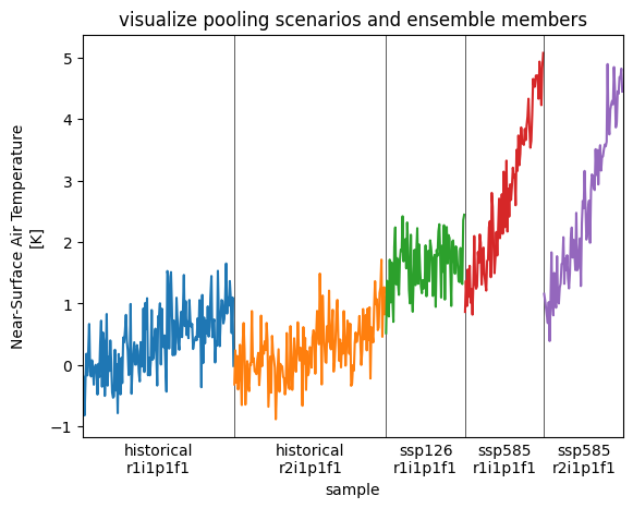
NCO: "4.6.0"Finally we pool all scenarios, and ensemble members into one dataset. Thies yields a Dataset where scenario, member, and time is pooled along a sample dimension. scenario, member, and time are kept as non-dimension coordinates, so we still know where each point comes from.
tas_pooled_y = mesmer.datatree.pool_scen_ens(tas_y)
tas_pooled_m = mesmer.datatree.pool_scen_ens(tas_m)

tas_pooled_y
<xarray.Dataset> Size: 585kB
Dimensions:   (gridcell: 118, sample: 588)
Coordinates:
    lat       (gridcell) float64 944B -49.5 -40.5 -31.5 -31.5 ... 76.5 76.5 76.5
    lon       (gridcell) float64 944B 288.0 288.0 18.0 ... 306.0 324.0 342.0
    scenario  (sample) object 5kB 'historical' 'historical' ... 'ssp585'
    time      (sample) object 5kB 1850-07-01 06:00:00 ... 2100-07-01 06:00:00
    member    (sample) <U8 19kB 'r1i1p1f1' 'r1i1p1f1' ... 'r2i1p1f1' 'r2i1p1f1'
Dimensions without coordinates: gridcell, sample
Data variables:
    tas       (sample, gridcell) float64 555kB -0.1548 -0.1209 ... 13.42 16.16
Attributes: (12/56)
    CDI:                       Climate Data Interface version 1.9.9 (https://...
    source:                    IPSL-CM6A-LR (2017):  atmos: LMDZ (NPv6, N96; ...
    institution:               Institut Pierre Simon Laplace, Paris 75252, Fr...
    Conventions:               CF-1.7 CMIP-6.2
    history:                   Thu Mar 18 19:05:09 2021: cdo remapbil,r20x20 ...
    creation_date:             2018-07-11T07:36:34Z
    ...                        ...
    realization_index:         1
    NCO:                       "4.6.0"
    cmip6-ng:                  \ncontact = cmip6-archive@env.ethz.ch\ndescrip...
    original_file_names:       /net/atmos/data/cmip6/historical/Amon/tas/IPSL...
    original_file_hash_codes:  7264c228560257b32d44dcc611d92976da7214af7e8795...
CDO: Climate Data Operators version 1.9.9 (https://...We visualize how the data is pooled:
def visualize_pooling(data):

    mi = pd.MultiIndex.from_arrays([data["scenario"].values, data["member"].values])

    data = data.assign_coords(sample=data.sample.values)

    f, ax = plt.subplots()

    xticks, xticklabels = [], []
    for i in mi.unique():

        loc = mi.get_loc(i)

        data.isel(sample=loc).plot()

        center = loc.start + (loc.stop - loc.start) / 2

        plt.axvline(loc.stop, color="0.1", lw=0.5)
        xticklabels.append("\n".join(i))
        xticks.append(center)

    ax.set_xticks(xticks)
    ax.set_xticklabels(xticklabels)
    ax.xaxis.set_tick_params(length=0)
    ax.set_title("visualize pooling scenarios and ensemble members")
    ax.set_xlim(0, data.sample.size)


visualize_pooling(tas_pooled_y.tas.isel(gridcell=0))
Calibration#
With all the data preparation done we can now calibrate the different steps of MESMER-M.
Fit the harmonic model#
First, we capture the seasonal cycle with a harmonic model. The coefficients of the model can vary with local annual mean temperature (fourier regression). This step removes the annual mean and determines the optimal order and the coefficients of the harmonic model: $$ T_{\text{mean response}}^{m,s,y} = \beta_{0,s} + \beta_{1,s} \cdot T_{s,y}
\sum_{i=1}^{n} \left[ g_{i,s}(T_{s,y}) \cdot \sin\left( \frac{i \pi (m \bmod 12 + 1)}{6} \right)
h_{i,s}(T_{s,y}) \cdot \cos\left( \frac{i \pi (m \bmod 12 + 1)}{6} \right) \right] $$, where the subscripts y,m and s denote year, month and spatial location.
harmonic_model = mesmer.stats.HarmonicModel()
harmonic_model.fit(tas_pooled_y.tas, tas_pooled_m.tas)

# we also need the residuals
harmonic_model_residuals = harmonic_model.residuals(tas_pooled_y.tas, tas_pooled_m.tas)

harmonic_model.params
<xarray.Dataset> Size: 26kB
Dimensions:         (gridcell: 118, coeff: 24)
Coordinates:
    lat             (gridcell) float64 944B -49.5 -40.5 -31.5 ... 76.5 76.5 76.5
    lon             (gridcell) float64 944B 288.0 288.0 18.0 ... 324.0 342.0
  * coeff           (coeff) int64 192B 0 1 2 3 4 5 6 7 ... 17 18 19 20 21 22 23
Dimensions without coordinates: gridcell
Data variables:
    selected_order  (gridcell) int64 944B 3 3 3 2 2 3 3 4 3 ... 2 4 4 3 3 3 2 4
coeffs (gridcell, coeff) float64 23kB -0.04407 4.653 ... nan nanApproximate the residuals#
The harmonic model does not capture all of the variance in the signal. The residuals (\(\eta_{m,s,y}\)), computed as the difference between the monthly temperature data and the harmonic model predictions, are approximated using probabilistic sampling strategies. This process has two steps: (i) ensuring the residuals follow a Gaussian distribution by applying a power transformer, (ii) approximating the transformed residuals as a multivariate AR(1)-process with a localised covariance matrix
Train the power transformer#
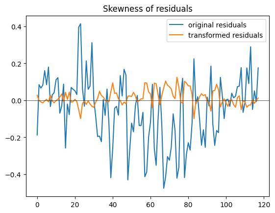
The residuals do no necessarily follow a gaussian distribution and might not be symmetric. Therefore, a Yeo-Johnson transformation is applied to map them onto a normal distribution:
The power transformer depends on a \(\lambda\) parameter that defines the transform. Normally, \(\lambda\) is constant, however, in Nath et al., 2022 \(\lambda\) is modelled with a logistic regression using local annual mean temperature as covariate: $\( \lambda_{m,s,y} = \frac{2}{1 + \xi_{0,m,s} \cdot e^{\xi_{1,m,s} \cdot T_{s,y}}} \)$
These two options are implements as "constant" and "logistic". We here use "constant" for performance reasons.
# Original Nath. et al version:
# yj_transformer = mesmer.stats.YeoJohnsonTransformer("logistic")

yj_transformer = mesmer.stats.YeoJohnsonTransformer("constant")
pt_coefficients = yj_transformer.fit(tas_pooled_y.tas, harmonic_model_residuals)
transformed_resids = yj_transformer.transform(
    tas_pooled_y.tas,
    harmonic_model_residuals,
    pt_coefficients,
)
To illustrate the effect of the transform, we plot the skewness of the original and the transformed residuals:
f, ax = plt.subplots()

ax.plot(
    sp.stats.skew(harmonic_model_residuals, axis=0),
    label="original residuals",
)
ax.plot(
    sp.stats.skew(transformed_resids.transformed.T, axis=0),
    label="transformed residuals",
)

ax.axhline(0, lw=0.5, color="0.1")
ax.legend()
ax.set_title("Skewness of residuals")
Text(0.5, 1.0, 'Skewness of residuals')
Fit cyclo-stationary AR(1) process#
The transformed monthly residuals (\(\tilde{\eta}_{m,s,y}\)) are now assumed to follow a cyclo-stationary AR(1) process, where the residuals in a given month depend on the residuals of the previous month and each month-to-month dependency has a distinct parameter: $\( \tilde{\eta}_{m,s,y} = \gamma_{0,m,s} + \gamma_{1,m,s} \cdot \tilde{\eta}_{m-1,s,y} + \nu_{m, s,y}, \\ \nu_{m, s,y} \sim \mathcal{N}(0, \Sigma_{\nu}(r)) \)$ Note that this means that individual months’ AR slopes can be outside [-1, 1], see github issue and Stroch and Zwiers (1999). Because there is no previous timestep for the first one, we loose one time step of the residuals.
AR parameters#
We first estimate the AR parameters through a regression
ar1_fit, ar1_residuals = mesmer.stats.fit_auto_regression_monthly(
    transformed_resids.transformed
)
ar1_fit
<xarray.Dataset> Size: 25kB
Dimensions:    (month: 12, gridcell: 118)
Coordinates:
  * month      (month) int64 96B 1 2 3 4 5 6 7 8 9 10 11 12
    lat        (gridcell) float64 944B -49.5 -40.5 -31.5 ... 76.5 76.5 76.5
    lon        (gridcell) float64 944B 288.0 288.0 18.0 ... 306.0 324.0 342.0
Dimensions without coordinates: gridcell
Data variables:
    slope      (month, gridcell) float64 11kB 0.1944 0.1468 ... -0.06053 0.08392
intercept (month, gridcell) float64 11kB -0.05807 -0.1008 ... 0.01934Find localized empirical covariance#
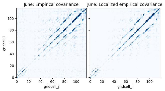
For the covariance matrix of the white noise we first estimate the empirical covariance matrix of the gridcell’s values and then localize it using the Gaspari-Cohn function. This function goes to 0 for for larger distances and becomes exactly 0 for distances twice the so called localisation radius. This is also called regularization. It ensures that grid points that are further away from each other do not correlate. Such spurious correlations can arise from rank deficient covariance matrices. In our case because we estimate the covariance on data that has more gridcells than timesteps.
The localisation radius is a parameter that needs to be calibrated and we find the best localisation radius by cross-validation of several radii using the negative loglikelihood.
We determine the localized empirical spatial covariance for each month individually.
prepare the distance matrix, i.e., the distance between the gridpoints in km
geodist = mesmer.geospatial.geodist_exact(tas_y.historical.lon, tas_y.historical.lat)
prepare the localizer(s) to regularize the covariance matrix
phi_gc_localizer = mesmer.stats.gaspari_cohn_correlation_matrices(
    geodist, localisation_radii=LOCALISATION_RADII
)
Compute the weights
weights = mesmer.weighted.equal_scenario_weights_from_datatree(tas_anoms_m)
weights = mesmer.datatree.pool_scen_ens(weights)

# because ar1_residuals lost the first ts, we have to remove it here as well
weights = weights.isel(sample=slice(1, None))
weights
<xarray.Dataset> Size: 395kB
Dimensions:   (sample: 7055)
Coordinates:
    scenario  (sample) object 56kB 'historical' 'historical' ... 'ssp585'
    time      (sample) object 56kB 1850-02-15 00:00:00 ... 2100-12-16 12:00:00
    member    (sample) <U8 226kB 'r1i1p1f1' 'r1i1p1f1' ... 'r2i1p1f1' 'r2i1p1f1'
Dimensions without coordinates: sample
Data variables:
weights (sample) float64 56kB 0.5 0.5 0.5 0.5 0.5 ... 0.5 0.5 0.5 0.5 0.5find the best localization radius and localize the empirical covariance matrix
The more samples we pass to
find_localized_empirical_covariance_monthly, the estimated localisation radius becomes larger. You may want to pass moreLOCALISATION_RADIIthan we do here (however, the function warns if either the smallest or largest localisation radius is chosen).Note that we fit the covariance matrix on the residuals of the cyclo-stationary AR process and not the power transformed residuals. This is because the variance of the time series we observe is bigger than the variance of the driving white noise process. For a standard AR(1) process (as employed in MESMER), this issue is mitigated by adjusting the covarinace matrix using the AR parameters. However, this approach cannot be employed for a cyclo-stationary AR(1) process. For details, see the corresponding github issue.
dim = "time"
k_folds = 30

localized_ecov = mesmer.stats.find_localized_empirical_covariance_monthly(
    ar1_residuals,
    weights.weights,
    phi_gc_localizer,
    dim=dim,
    k_folds=k_folds,
)
# plot the localized covariance matrix against the empirical covariance matrix for the month of June
month = 6

f, axs = plt.subplots(1, 2, sharey=True, constrained_layout=True)

opt = dict(vmin=0, vmax=1.5, cmap="Blues", add_colorbar=False)

ax = axs[0]
localized_ecov.sel(month=6).covariance.plot(ax=ax, **opt)
ax.set_aspect("equal")
ax.set_title("June: Empirical covariance")

ax = axs[1]
localized_ecov.sel(month=6).localized_covariance.plot(ax=ax, **opt)
ax.set_aspect("equal")
ax.set_title("June: Localized empirical covariance")
ax.set_ylabel("")
plt.show()
Saving the parameters#
Finally, we have calibrated all needed parameters and can save them. We can use filefisher to nicely create file names and save the parameters.
# define path relative to this notebook & create folder
param_path = pathlib.Path("./output/calibrated_parameters/mesmer-m/")
Create time coordinate#
We overwrote the time coordinate with ‘sample’. Thus, we need to get the original time coordinate to be able to validate our results later on. If it is not needed to align the final emulations with the original data, this can be omitted, the time coordinates can later be generated for example with
monthly_time = xr.cftime_range("1850-01-01", "2100-12-31", freq="MS", calendar="gregorian")
monthly_time = xr.DataArray(monthly_time, dims="time", coords={"time": monthly_time})
hist_time = tas_m.historical.time
scen_time = tas_m.ssp585.time
m_time = xr.concat([hist_time, scen_time], dim="time")
Store data for all modules#
PARAM_FILEFINDER = filefisher.FileFinder(
    path_pattern=param_path / "{esm}_{scen}",
    file_pattern="params_{module}_{variable}_{esm}_{scen}.nc",
)

scen_str = "-".join(scenarios)

folder = PARAM_FILEFINDER.create_path_name(esm=model, scen=scen_str)
pathlib.Path(folder).mkdir(exist_ok=True, parents=True)


# NOTE: to save disk space the "covariance" can be removed from localized_ecov
localized_ecov = localized_ecov.drop_vars(["covariance"], errors="ignore")

params = {
    "harmonic-model": harmonic_model.params,
    "power-transformer": pt_coefficients,
    "local-variability": ar1_fit,
    "covariance": localized_ecov,
    "grid-orig": grid_orig,
    "monthly-time": m_time,
}

save_files = False  # we don't save them here in the example
if save_files:

    for module, param in params.items():

        filename = PARAM_FILEFINDER.create_full_name(
            module=module,
            esm=model,
            scen=scen_str,
            variable=variable,
        )

        param.to_netcdf(filename)